[ Home ] [ Up ] [ Introduction to Excel ] [ Entering a Range of Data ] [ Formatting Cells to Match Data Types ] [ Cut, Copy, Paste and Move Data ] [ Inserting and Deleting Rows and Columns ] [ Entering and Replicating Formulas ] [ Using Simple Functions ] [ Producing Charts with Labels ] [ Printing Selected Areas ]

Using Simple Functions

Functions are more powerful than simple formulas.  For instance if you wanted to add a range of numbers such as cells A14 through K14 you would have to type =A14+B14+C14...+K14.  To do this more simply you could use a function =SUM(A14:K14), this would tell Excel to sum all of the data from cells A14 through K14.

Manually Entering the SUM Function

Automatically Entering the SUM Function

Manually Entering the AVERAGE Function

Automatically Entering the AVERAGE Function

Changing Functions

Copying Functions Using the Fill Handle

Copying Functions using Copy and Paste

Using Multiple Formulas

Showing Formulas and Functions

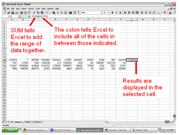
Manually Entering the SUM Function

Follow these instructions if you want to add all of the numbers in a range together.

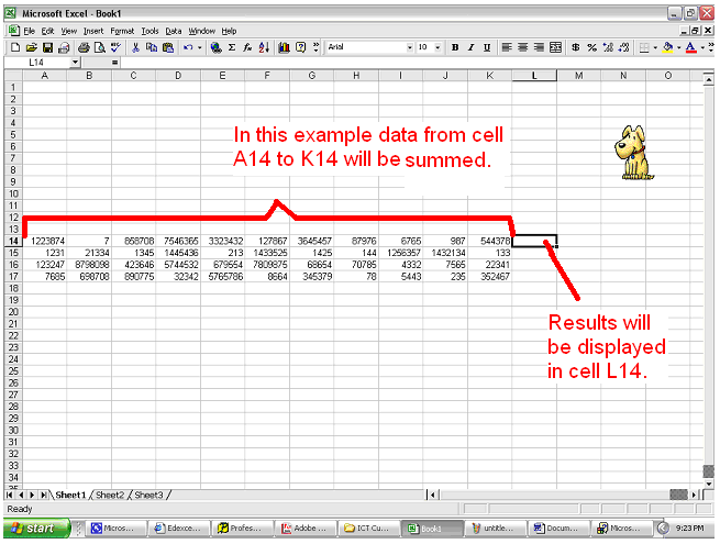
1. Click on the cell where you want your results to be displayed.
2. Click on the formula bar and type an = sign.
3. Type AVERAGE(A14:K14) then press the enter key.

SUM tells Excel to add the numbers from the cells in the brackets.  By typing a colon (:) between the cell references you are telling excel to include all of the cells between these cell references.

If you want to add several numbers together that are not close to each then you use commas in between the cell references.  For example, if you wanted to total B14, F14, and J14, you would type =SUM(B14,F14,J14)

4. The results should be displayed in the cell you have chosen.

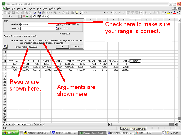
Automatically Entering the SUM Function

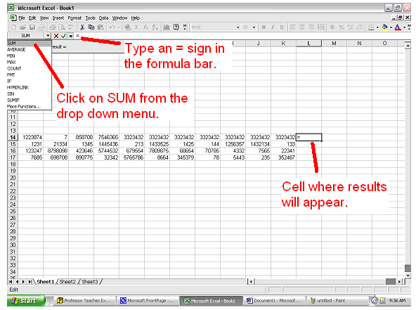
1. Click on the cell in which you wish your results to appear.
2. Click in the formula bar and type an = sign.  The cell reference menu will turn into a 
   Function Menu.
3. Click on the Function Menu and click on SUM.
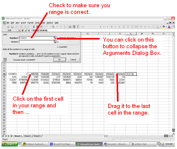
4. The Function Arguments Dialog Box will appear.  Check to make sure the range is correct and then Click on OK.                                                                                                                     
5. If your range is not correct click and hold on the first cell in your range then drag the box to the last cell in your range.  Click on OK when you are satisfied.                 

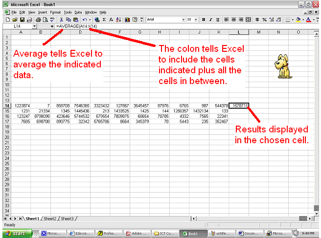
Manually Entering the AVERAGE Function

Sometimes you may want to total or find the average of a long list of numbers.  In order to do this you will need to use a function.

See the example below:

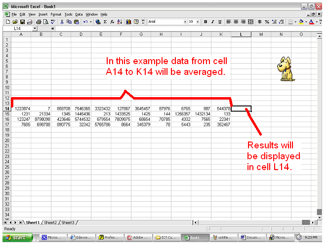
1. Click on the cell where you want your results to be displayed.
2. Click on the formula bar and type an = sign.
3. Type AVERAGE(A14:K14) then press the enter key.

AVERAGE tells Excel to average the numbers from the cells in the brackets.  By typing a colon (:) between the cell references you are telling excel to include all of the cells between these cell references.

4. The results should be displayed in the cell you have chosen.

Automatically Entering the AVERAGE Function

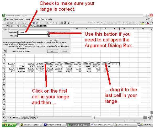
1. Click on the cell in which you wish your results to appear.
2. Click in the formula bar and type an = sign.  The cell reference menu will turn into a
   Function Menu.
3. Click on the Function Menu and click on AVERAGE.
4. The Function Arguments Dialog Box will appear.  Check to make sure the range is correct and then Click on OK.                             
5. If your range is not correct click and hold on the first cell in your range then drag the box to the last cell in your range.  Click on OK when you are satisfied.

Changing Functions

If you want to change the function you have chosen but not your range then do this:

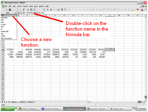
1. Double click on the function name in your formula bar.
2. Click on the Function Drop Down Menu.
3. Choose a new function.                   
4. The Arguments Dialog Box will pop-up.  Check your range and Click on OK.

Other Functions

Other functions are entered in much the same way as SUM and Average, therefore only explanations of the other functions will ensue.

COUNT: counts the number of pieces of data in a range.

MAX: tells you the largest number in your range.

MIN: tells you the smallest number in your range.

Copying Functions Using the Fill Handle

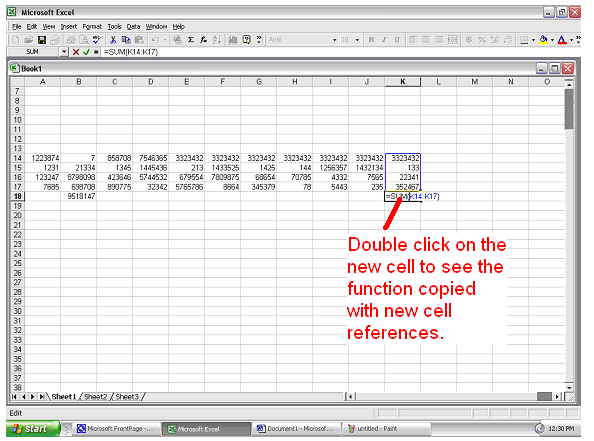
If you want to use the same formula with different cell references in a new cell then follow these instructions.

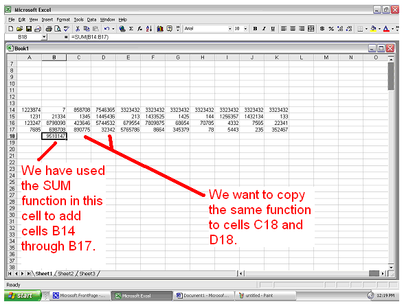
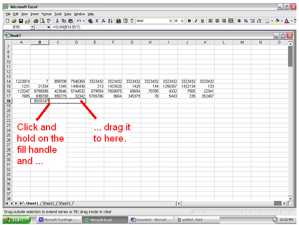
1. Click in the cell with the function you wish to replicate.
2. Click and hold on the fill handle and drag to the cells where you wish to copy the function.
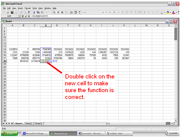
3. Release the mouse button and the formula should be copied with the new cell references.  Double click on the new cell to make sure your formula is correct.

Copying Functions using Copy and Paste

Sometimes you may want to copy functions to cells that are not adjacent to each other.  For example,                                               

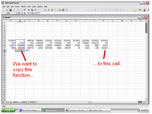
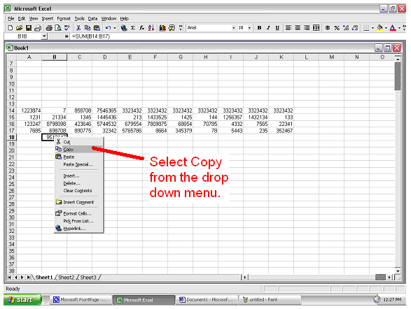
1. Right click on the cell with the function you want to copy and select Copy from the drop down menu.                                             
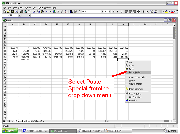
2. Right click on the cell you wish to copy the formula to and click on paste special.
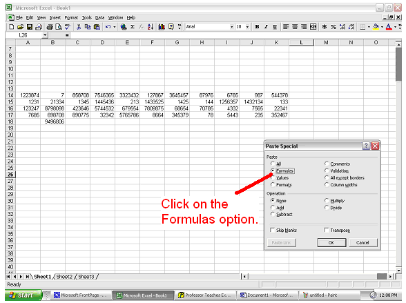
3. Click on the Formulas option in the dialogue that pops up then click O.K.
4. Double click on the new cell to make sure the formula is correct.

Using Multiple Formulas

You will find several cases in which you may have to use more than one calculation at a time.  For example you may want to add a column of numbers and then multiply it by ten. 

When you do this you have to make sure that you are following the order of operations.  When you have a long calculation you need to complete whatever is in brackets first, then any exponents, then any division or multiplication, then addition or subtraction.

A good way to remember this is by using the acronym BEDMAS. 

B: Brackets first

E: then Exponents

D: then Division

M: or Multiplication

A: then Addition

S: or Subtraction

For example in the equation:

Showing Formulas and Functions

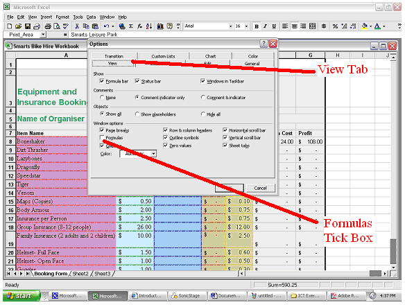
To show all the formulas on a spreadsheet do this:

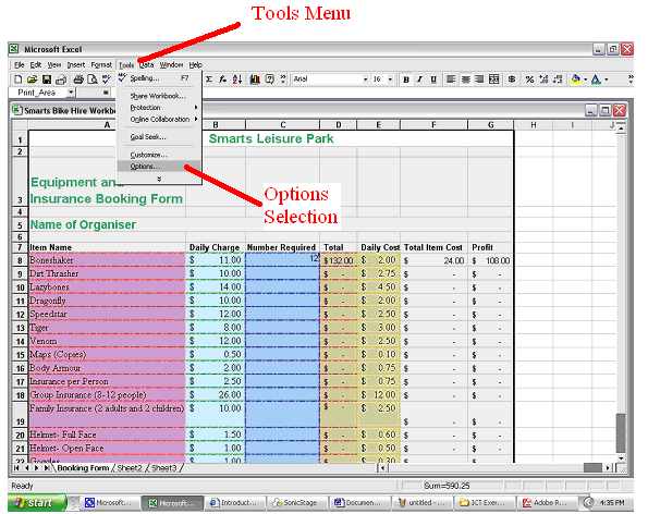
1. Open the Tools menu on the Standard Toolbar and click on Options.
2. Click on the View tab of the dialogue box which opens up and tick the Formulas box.