
Applications of |
 See this page's Maple Code |
I. Distance from a Point to a LineIn our first application we will find the minimum distance from a point to a line in 3-space. We will use the point  and the line defined by the vector equation and the line defined by the vector equation  , both shown in the graph on the right. , both shown in the graph on the right.This shortest possible distance will be represented by the segment AB, where the point B is on l. (See the green segment below, with our viewing angle adjusted slightly.) We need to find the orthogonal distance, since this will be the minimum distance; this means that AB and l must be perpendicular. Therefore, if we can derive two vector equations, we can then use the fact that their dot product must be zero to find the shortest possible distance from A to l. We will go through the process step by step, and then look at how Maple makes the task slightly easier. |
|
 . In the same way, the segment AB can be represented by the vector from A to B, and that vector is
 |
 . Substituting back in vector AB's equation gives us . Substituting back in vector AB's equation gives us
 , and the magnitude of this is , and the magnitude of this is
to is 3.
|
 |
|
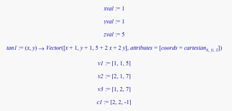
II. Finding A Normal Vector and Tangent Plane to a SurfaceIn two-dimensional calculus, we can use the derivative to find the formula of a tangent to a curve at any given point on the curve. When we extend that idea to three dimensions - meaning, we look at tangents to surfaces then the derivatives become more complex. There are "partial" derivatives, "directional" derivatives, "gradients," "normal vectors" and tangent planes instead of tangent lines.In this application we will find the equation of the plane tangent to the surface of  at the point at the point  . To do so, we will find the directional derivatives along the x- and y-axes; then translate those derivatives into vectors with base ; then take the cross product of those vectors to find the "normal" vector to the surface; and, finally, use that normal vector to find the tangent plane's equation. . To do so, we will find the directional derivatives along the x- and y-axes; then translate those derivatives into vectors with base ; then take the cross product of those vectors to find the "normal" vector to the surface; and, finally, use that normal vector to find the tangent plane's equation.
|
First we take the partial derivatives of z: Since these tell us how fast z is changing with respect to the two variables, we can plot the tangent vectors  and and  , ,where the z-component is found by substituting x=1, y=1 into each directional derivative's formula. This gives us the tangent vectors shown in red on the right: each has endpoint (1,1,5), and they represent change in the xz- and yz-planes. Finally, we can calculate the plane's equation by using the cross product of these two partial derivatives. Since each derivative is tangent to the surface, the cross product will be normal to the surface (since it will be perpendicular to the plane of dz/dx and dz/dy, which is itself tangent to the surface). The normal vector will then give us the equation of the plane. The process is identical to the process on the "Three-Dimensional Vectors" page; we can also use the Maple code shown below. |

|
 |
 shown in blue below left. To its right, we add the tangent plane, whose equation is
  (with the constant value of -1 found by substituting (1,1,5) into the vector formula 2x+2y-z).
|  |
| We can also calculate and plot a tangent plane by using Maple's "Tangent Plane" function, as in the code block below; note that we still have to convert the tangent plane output into a graphable form. (See the Maple worksheet for the graph created by this program.) | |
  | |
| By rotating the view we see that the blue vector is in fact normal, and the plane tangent, to the paraboloid at point A. Click here for the Maple animation code | 
|
| > restart:with(plots):with(linalg): > with(VectorCalculus):SetCoordinates('cartesian'[x,y,z]): > C:=NULL:B:=NULL:F:=NULL:for n from 1 to 9 do xval:=sqrt(10)*(n-1)/16:yval:=sqrt(10)*(n-1)/16:zval:=xval^2+yval^2+3: tan1:=TangentPlane((x,y)->x^2+y^2+3, xval,yval):pt1:=subs(x=0,y=0,tan1(x,y)):pt2:=subs(x=1,y=0,tan1(x,y)):pt3:=subs(x=0,y=1,tan1(x,y)): > v1:=convert(pt1,vector):v2:=convert(pt2,vector):v3:=convert(pt3,vector): > c1:=crossprod(evalm(v3-v1),evalm(v2-v1)):C:=C,plot3d({x^2+y^2+3,c1[1]*x+c1[2]*y-(c1[1]*xval+c1[2]*yval+c1[3]*zval)},x=-3..3,y=-3..3, view=-16..16,axes=normal,orientation=[20,75]): xval2:=sqrt(5)*cos(Pi/4-Pi*(n-1)/32):yval2:=sqrt(5)*sin(Pi/4-Pi*(n-1)/32):zval2:=xval2^2+yval2^2+3:tan2:=TangentPlane((x,y)->x^2+y^2+3, xval2,yval2): pt4:=subs(x=0,y=0,tan2(x,y)):pt5:=subs(x=1,y=0,tan2(x,y)):pt6:=subs(x=0,y=1,tan2(x,y)): > v4:=convert(pt4,vector):v5:=convert(pt5,vector):v6:=convert(pt6,vector): > c2:=crossprod(evalm(v6-v4),evalm(v5-v4)):B:=B,plot3d({x^2+y^2+3,c2[1]*x+c2[2]*y-(c2[1]*xval2+c2[2]*yval2+c2[3]*zval2)}, x=-3..3,y=-3..3,view=-16..16,axes=normal,orientation=[20,75]):xval3:=sqrt(5)*(8-n)/8:yval3:=0:zval3:=xval3^2+yval3^2+3: tan3:=TangentPlane((x,y)->x^2+y^2+3, xval3,yval3):pt7:=subs(x=0,y=0,tan3(x,y)):pt8:=subs(x=1,y=0,tan3(x,y)):pt9:=subs(x=0,y=1,tan3(x,y)): > v7:=convert(pt7,vector):v8:=convert(pt8,vector):v9:=convert(pt9,vector): > c3:=crossprod(evalm(v9-v7),evalm(v8-v7)):F:=F,plot3d({x^2+y^2+3,c3[1]*x+c3[2]*y-(c3[1]*xval3+c3[2]*yval3+c3[3]*zval3)}, x=-3..3,y=-3..3,view=-16..16,axes=normal,orientation=[20,75]):od:display(C,B,F,insequence=true); |
 Click here for the animation's Maple worksheet |
|
 Return to Main Vector Page |
 Go to 2-D Vector Page |
 Go to 3-D Vector Page |

 .
. .
. .
.