Learning LT Spice.
Lesson 5

Click here to download a PDF of this page.

Table of Contents.

Lesson 1: Fundamental Drawing Skills and a Simple Simulation.
Lesson 2: Introduction to Frequency and transient Analysis.
Lesson 3: Configuring LT Spice and more Drawing controls.
Lesson 4: Locating, modifying, and installing vacuum tube models.
Lesson 5: Operating point of vacuum tube circuits. Introduction to stepping and plate curves. This page.
Lesson 6: Finding, installing, and using, potentiometer symbols and models.
Lesson 7: Transient analysis of unregulated power supplies.
Lesson 8: Transient analysis of power supply regulators.
Lesson 9: Transient and frequency analysis of amplifiers with feedback.
Lesson 10: Lossless transformers.
Lesson 11: Making symbols and models.

Lesson 5
Operating point of vacuum tube circuits.
Introduction to stepping and plate curves.

What you will learn in Lesson five. How to:

1. (Review) Retrieve a Previously Saved file.
2. (Review) Use Drag Mode.
3. (Review) Determine the DC operating point of the tube in a resistance coupled amplifier.
4. (Review) Run the frequency response of the R C amplifier.
5. Call up cursors for highly accurate readings of specific points on the curve(s).
6. Find the Vout / Vin gain of the R C amplifier.
7. Examine how changing the value of the coupling capacitor effects low end frequency response.
8. Examine how adding a cathode bypass capacitor increases the gain and its effect on the low end.
9. Compare an R C amplifier with different tube types plugged in.
10. Build a simulated curve tracer for plate characteristics
11. Measuring rp, Gm, and μ, of a tube model and comparing them with tube manual values.
12. Avoid misinterpretation of results when two graphs look the same but aren't.

.

Having trouble remembering all those syntaxes?
Here's a summary page that should help.

Control click on this link to open it in a new window. Control Tab will switch back and forth between the current lesson page and this help page.

Retrieving a Previously Saved file.

Load the file you saved at the end of the last lesson. If you took my advice you would have named it "Lesson-04-01". If you named it something else it's up to you to find it, I can't help you. Presumably you now have this figure showing in LTspice.

Figure 5.1.1 Simple Triode Amplifier before changing cathode resistor.

Change the value of R1 from 1.8 k to 3.3 k and change the" .ac" spice directive from a directive to a comment. Here's how. 1. Right click on the ".ac" directive. 2. After the dialog box comes up press the ESC key. 3. You will now see this.

Figure 5.1.2 Cathode resistor changed and dialog box showing how to convert a directive to a comment.

4. Click the radio button in front of the word "Comment" and click OK.

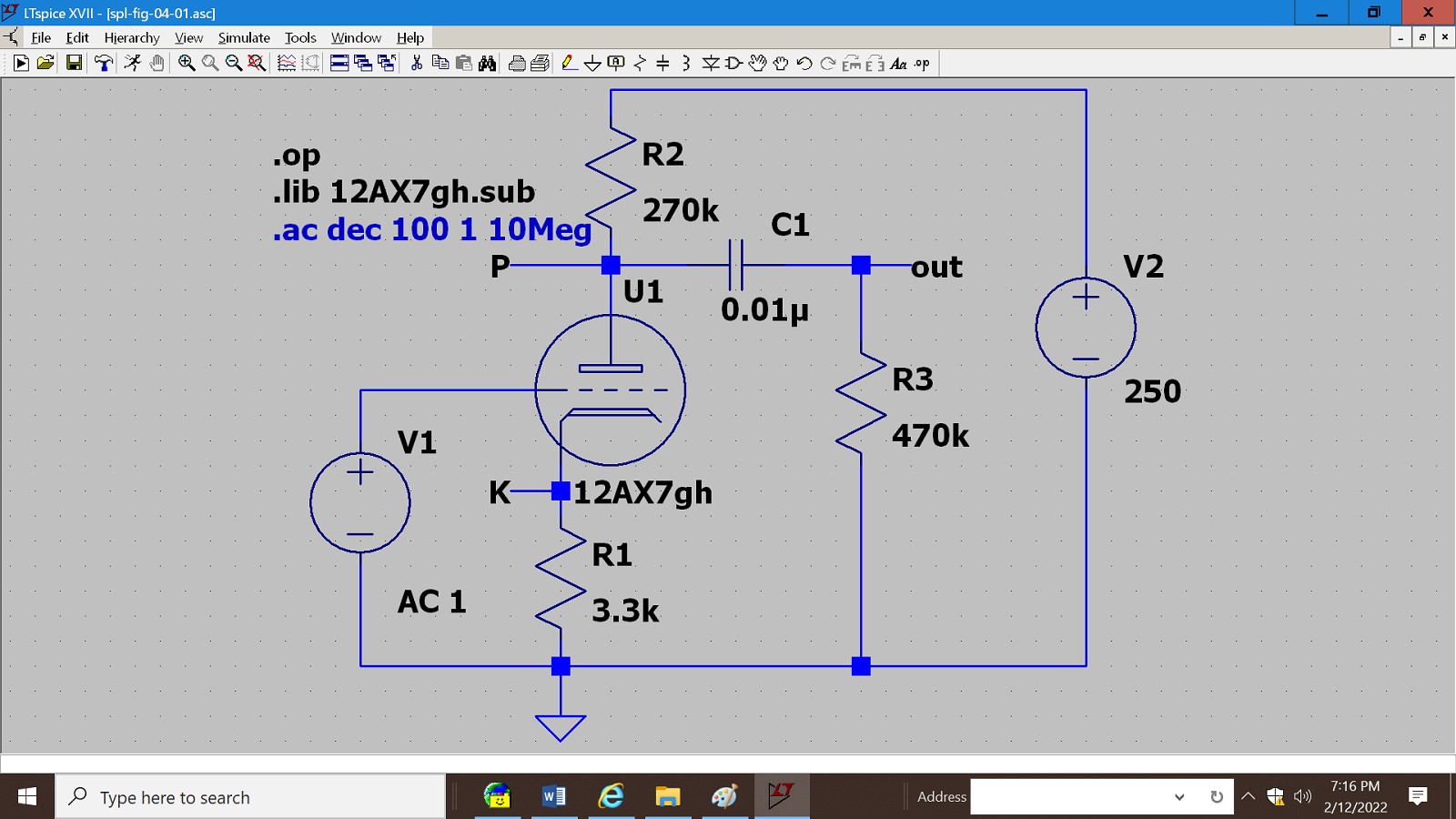
Figure 5.1.3 ".ac" directive changed to a comment.

And then save the circuit as slp-fig-05-01.

(Note: Other sources are likely to tell you to edit the text of the directive by deleting the period (.) and replace it with a semicolon (;). Like the color change, the semicolon tells spice to treat the line of text as a comment and not to do what it directs. I see several advantages to changing the color rather than editing the text. First of all there is really no need to delete the period because everything after a semicolon is a comment and it doesn't matter what follows it. Second the color change is much more eye catching than the semicolon and when your simulation won't run you will be much more likely to see that the directive has been deactivated by turning it into a comment.

Using Drag Mode.

A cathode bypass capacitor is needed for some of the simulations we are going to do. As currently drawn there isn't room to connect it at the cathode of the tube while keeping the diagram neat. So we will review the Drag command. To give yourself a little more room to work press ctrl-B to pull back the zoom. Drag is in the Edit Menu and is the closed hand on the tool bar. It can also be invoked by pressing F8. To execute the drag command, after pressing F8 you press and hold the left mouse button and draw a box as shown below. Hint, start with the lower left corner and allow plenty of room to include the ground. Set the upper right corner so the dashed line is just above the horizontal line as shown. Make sure the dashed line crosses the bright blue line that leads to R1. If it crosses the dark blue line the resistor will be disconnected. Release the button and move the mouse downward. The bottom line and ground symbol will move downward and probably a little to the left or right. The lines connecting to the two generators and two resistors will stretch but remain connected.

Figure 5.2 Preparing to move bottom line and ground.

When you have everything lined up and where you want it, left click and they will be fixed in place. You can see the end result in figure 5.3.1.

Again press F8 and draw a box around R1 as shown in figure 5.3.1. It is important that the dashed lines cross the bright blue lines of the wires not the dark blue leads of the resistor.

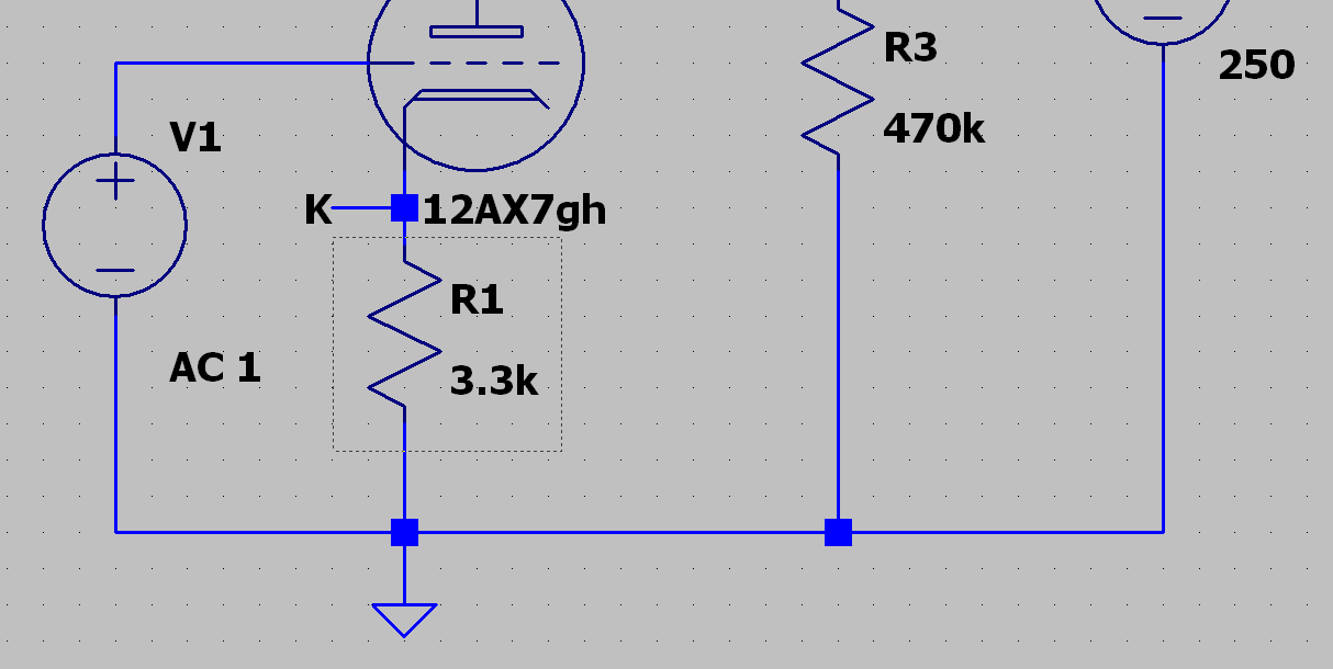
Figure 5.3.1 Results of moving bottom line and preparing to move R1.

As you move the mouse you will see the connecting leads stretch but not disconnect. Position the bottom end of the resistor a couple of jumps up from the bottom line and click. There is now enough room to connect a capacitor across the resistor. We will do that later.

Determining the Operating Point.

Notice that the ".op" directive was active when running the ".ac" simulation. No harm is done by leaving it active. Press F10 to run the simulation.

Figure 5.3.2 Results of running the operating point.

Using "Net Name" to name nodes.

Now you see the reason we have used "net name" to assign P and K to the plate and cathode respectively of the tube. The listing includes V(n001) and V(n002) but there is no way to tell where these nodes are located and no way to make LTspice place these labels on the schematic. The only way to get at these numbers is to call up the "netlist". But unless you have been a spice user since the FORTRAN days you probably won't know how to interpret it. Our lifeline is the "Net Name" feature. We have given our own names to the plate, cathode, and amplifier output. These have replaced node numbers in the netlist and on the listing of node voltages. Thus what was previously hidden becomes clear to us. Notice that the listing includes V(p) = 134.8 volts and V(k) = 1.408 volts. I have rounded off these values. I haven't yet found a way to make LTspice round off the printed values. There may not be a way.

If you have time you might want to try different models to see if they yield different results.

Running the frequency response.

Right click on the AC directive and re enable it by clicking the "SPICE directive" radio button. There is no need to disable the op directive. Press F10. If the graph is blank, look at the borders of the schematic and graph windows. If the border of the schematic is a much lighter blue than the graph, click on the top border of the schematic. It will turn to a darker blue. If it is already dark you don't need to click it.

Now move the mouse into the schematic area. Move it over the line leading to the word "out". The cursor will turn into a scope probe. Click on the line. The graph lines will appear along with scales and numeric labels. You will see the amplitude expressed in dB and phase plotted versus frequency. Eyeball interpolation gives the mid band gain as 29 dB. Mid band phase is the expected 180 degrees.

Press control S to save the schematic. Click on the border of the graph. Press control S again to save the settings of the graph including where the scope probe is connected. If you remember to do this, it may not have to be done again.

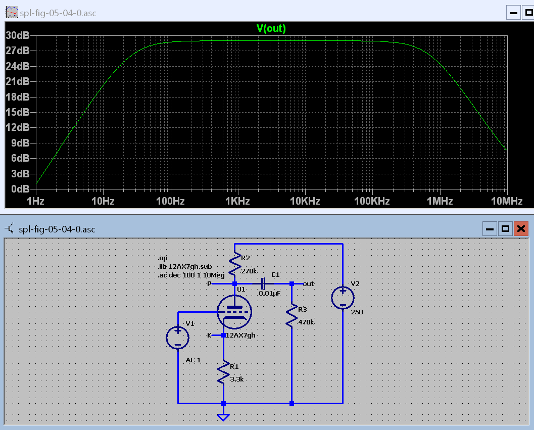
Figure 5.4.0 Frequency response over a wide range.

Unless I'm particularly interested in phase values I find the phase graph to be confusing. If you agree, move the mouse over the right hand vertical scale. The cursor will turn into a ruler. Right click and a dialog box will come up. Click on the "Don't plot phase button. The dialog will close and the phase will be gone.

Cursors for Accurate Readings.

Look at the top center of the graph window and find the legend "V(out)" in green. Click on it. Two crossed white lines will appear on the graph and a readout box will appear in the lower right area of the screen. This is the cursor function which is found on most digital oscilloscopes these days. Position the mouse over the vertical line and a yellow "1" will appear. Hold and drag to move the cursor to any frequency. The readout box will give you the frequency, the amplitude, phase, and just for good measure the group delay. Have fun with this one. To get out of this click the X in the upper right corner of the readout box. You can call up a maximum of 2 cursors.

To call up the second cursor first move cursor 1 away from the place where it appeared so you can tell when the second one appears. Now click on the "V(out)" legend again. The second cursor will appear and the blank boxes in the cursor window will be filled in. When you hover over the vertical line of the second cursor a yellow "2" will appear.

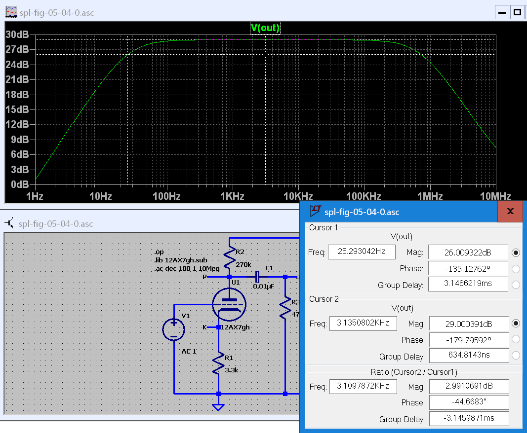
Figure 5.4.1 Using cursors to find one of the 3 dB down frequencies.

Move either cursor down so it is on the low end slope as shown in the screen shot above. Adjust the frequency by moving the cursor until the "Mag." (magnitude) reading for that cursor is as close to 26 dB as you can get it, 3 dB down from 29.00 dB. You will never get all 8 digits to match up so don't waste your time trying. The frequency is 25.3 Hz which isn't too bad but not good enough for high fi fans.

Finding the V(out) / V(in) of the amplifier.

This is an area where the terminology gets a little fuzzy. What is shown above is the gain in dB. When engineers and technicians say "gain" they generally mean the output voltage divided by the input voltage. Because this is a voltage divided by a voltage it has no dimensions. It is not the gain in anything, it is just the gain. If you have a science and engineering calculator you can calculate the gain from gain in dB with just a few keystrokes. But if you don't have one and you are curious you might want to know how to make LTspice tell you.

Move the cursor over the graph area and click anywhere. Move it to the dB scale on the left. It will turn into a ruler. Right click and in the box that opens click the "linear" radio button. While you are there change the top value to 30, the tic value to 3 and the bottom value to 0 and then OK. LTspice is not particularly rigorous about units. This is actually the output voltage but we have set the input voltage at 1 volt by setting the magnitude of the generator. So the gain and output voltage are numerically equal.

Figure 5.4.2 Using linear scale and cursors to find Vout/Vin.

Don't be troubled by the close values of gain in dB and Vout/Vin. Whenever there are two scales of values that are related by a function the possibility exists that there may be a point where the two scales have the same numerical value. A well known example are the two temperature scales. Fahrenheit and Celsius thermometers will read the same at -40 degrees.

C1 and Low End Frequency Response.

Right click on the capacitor C1 and change the value from "0.01u" to "{C1}" These are called braces.
Right click on the ".ac" directive and change the frequency to start = 1, and stop = 100. Then click OK.
Call up the spice directive window by typing the letter "S". Type ".step" and click OK.
Position the word where you want it and click. I suggest above V1 and above the line connecting R2 to V2.
Click to drop it there. Then right click on the word. In the dialog box set "Name of parameter to sweep" to "C1" without the braces.
Press TAB and set the "Nature of sweep" dropdown list to "List">
Press TAB again and in the "First value" type "0.01uf".
Press TAB again and in the "second Value" type "0.022uf".
Set "Third value" to "0.047uf".
Although you are out of boxes you aren't out of values. Press TAB one more time and you will be in the syntax box at the bottom of the dialog box.
DON'T PRESS ANY LETTER OR NUMBER KEYS! If you do the whole thing will be erased and you will have to start over. Press the right arrow.
The cursor will now be after the last uf. Press the space bar and continue typing values separated by spaces.
"0.1uf 0.22uf 0.47uf"
Click OK. The directive will be in the same place it was and will be complete.

Figure 5.4.3 Using ".step" directive to find best value for C1.

Press F10. The graph will probably be blank. Click on the output line again.
Click on the graph and press ctrl-S to save the connection.
The phase information is a bit confusing so right click on the right hand vertical scale and click on "Don't plot phase information".
You now have a plot of frequency response from 1 to 100 Hz for 6 different values of capacitor C1. Obtaining this information from a breadboard would be somewhat tedious. The green line is for C1 = 0.01 uF, blue for 0.022 uF and so on. To increase the usefulness of this graph you will restrict its range even more.

Adjusting the scales of a graph.

1. If there is little useful information below 10 Hz Do this.
2. Move the cursor over the frequency scale at the bottom. It will turn into a ruler.
3. Right click and set new values for the frequency scale. 10 for Left, 10 for Tic, and 100 for Right. Click OK. LTspice will add the Hz for you.
4. You can't go outside of the range set in the ".ac" directive. No data has been collected for those frequencies.

5. Now right click on the left hand vertical scale.
6. Set the values as follows. 30 for Top, 1 for Tic, and 20 for Bottom. You don't have to put in the dB. Spice will add them for you.
7. Press ctrl-S to save the graph settings.

Looking at the gain values at 20 Hz it is clear that there is a large improvement by going from 0.01 uF to 0.022 uF, and a little more than a dB improvement in going from 0.022 to 0.047 uF. But it seems pointless to go above 0.1 uf. However it must be born in mind that if you have a preamplifier with 3 or 4 such stages in a row that the attenuation at 20 Hz will be 3 or 4 times that for a single stage.
This is an example of the kinds of insights that LTspice can give you that you couldn't easily get from a breadboard.

Adding a cathode bypass capacitor.

Set the value of C1 to a fixed value of 0.1 uf and connect a cathode bypass capacitor from the top of R1 to ground. The added capacitor will be C2.
The value of C2 must be {C2}.
You need to change C1 to C2 in the ".step" directive.
Edit the ".step" directive to step C2 from 2.2 uF to 47 uF in the sequence that should now feel familiar, 2.2, 4.7, 10, etc.
Run the simulation.
Note the gain values at 20 Hz. Tip: after you run the simulation your scale settings may go away but if they did, they haven't gone far. Right click on the graph area and hover over the "File" entry almost at the bottom of the menu. Click "Reload Plot Settings" in the sub menu that pops up. If the settings don't come back don't feel bad. You may have forgotten to save them. The frequency scale should go from 10 to 100 Hz. If it goes from 1 to 100 Hz perform the steps under the heading "Adjusting the scales of a graph." Which is just before the heading "Adding a cathode bypass capacitor."

Here are the results of stepping the cathode bypass capacitor. With C1 set to 0.1 uf.

Figure 5.5 Using ".step" directive to find best value for C2.

Using cursors with multiple curves.

Click on the "Vout" legend. Move the cursor away from the place where it appeared and click the legend again. It's on the same curve isn't it. OK let's start over. Click in the upper right corner of the readout box to close it.

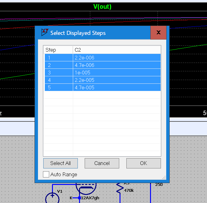
Figure 5.5.1 Navigating steps.

Right click anywhere in the graph area. In the menu that comes up hover over "View" and in the sub menu click on "Select steps". What you will see will be similar to figure 5.5.1.
Uncheck the box labeled "Auto Range". Watch this, it has a way of coming back. It will mess up your scale settings.
Click on row 5 and the selection of all other lines will be switched off leaving only number 5 selected.
Click OK.
Click on the "Vout" legend.
This will create a cursor that will track curve 5, .
Move it out of the way near 40 Hz.
Once again right click anywhere on the graph to open the context menu.<
Hover over "View" and click "select steps".
Hold the control key and click row 3.
You should see something similar to figure 5.5.2.
Uncheck "Auto Range" and click OK.

Figure 5.5.2 Navigating steps.

Now click the "Vout" legend again.
You should see something like Figure 5.5.3.
The second cursor should track the red line.

Figure 5.5.3 Navigating steps.

Move cursor number 1 to 100 Hz.
Move cursor number 2 to 20 Hz.
The cursor values given in the box are much more accurate than you could get by reading the graph.
Cursor number 1 is reading a value very close to the mid band gain of the amplifier. You will notice that the red line gives a value which is 1 dB down from mid band to an accuracy of 1/100 of a dB. That's quite a lot of overkill when you remember that a dB is the change that the human ear can just barely manage to detect. I promise I didn't cherry pick these values. I set it up with standard component values and let the microfarads fall where they may.

If you have forgotten which capacitor value the red line represents you may have already noticed the item that comes right after "Select Step". It is "Step Legend". It says in purple 47 u and in red 10 u.

Granted, this is a complicated procedure and if you get a single step wrong it won't come out right at the end. But it can be used for any condition where you have multiple curves on a graph and you need to know their values with some accuracy.

What Happens if you Plug in a Different Tube.

This is a question often asked by the uninitiated. They are told "in general don't do it. You could do damage to the tube or device you are plugging it into or both." But in the case of the 12 volt dual triodes you can plug away as long as it doesn't have series strung heaters. The operating point might be a little off but it may not matter.

So let's clone our little amplifier circuit and see what damage we can do. First we need to decide what part to clone. Figure 5.6 shows a selection box that was drawn after pressing ctl-C.

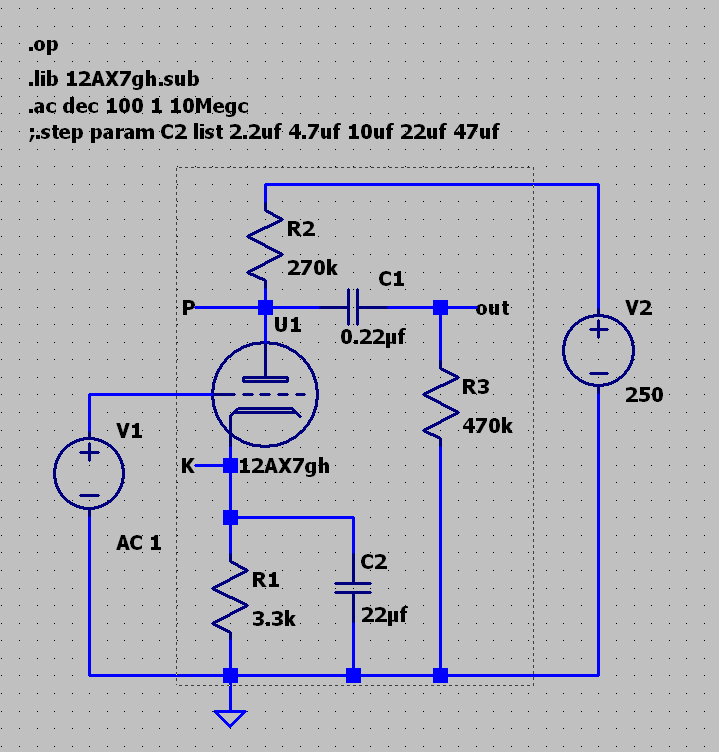
Figure 5.6 Showing a portion of the diagram selected to be copied.

After you release the mouse button after drawing the box you might think that nothing happened. Move the mouse a little. See? You have the tube along with associated resistors and capacitors. Move it over to the right and click to put it in its place as shown in figure 5.7. This doesn't work quite like copy and paste in a word processor where you can paste as many times as you want from one ctrl-C. Again press ctrl-C and again draw a box round the tube and parts you just placed. Again after you release the mouse button you will have a copy of it under mouse control. Place it to the right of the one you just placed. You can actually do this as many times as you have tubes you want to compare. As you can see by the figure I started with 4 test positions. But I really wanted to compare 6 of the 12 volt dual triodes.

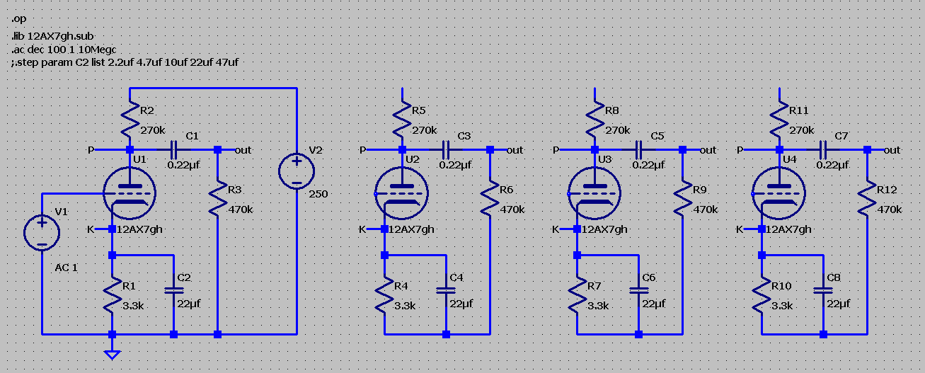
Figure 5.7 Showing the diagram after the tube circuit has been copied.

So we need to fix it in Figure 5.8 by adding two more clones. Then draw in the leads to connect the common points and the B+ points. Then draw a lead to connect the other three grids to the generator V1. Also we will move generator V2 out of the line to keep the diagram from getting too long.

Houston, we have a problem.

The labels "P", "K", and "out" aren't unique. LTspice will interpret this as, all points labeled P are to be connected together, all points labeled K are to be connected together, and all points labeled out are to be connected togetther. All you would get from this is all of the tubes connected in parallel. This is not what we want.

LTspice assumes this is what you want to do. If you want them to be separate you must assign individual numbers to each occurence of P, K, and out. Just right click on each one and append a number, 1, 2, 3, etc, after the letter or word.

Figure 5.8 Gain comparison of 6 of the most common dual triode tubes. I wonder what happened to the 12AW7?

Checking the operating point isn't hard, just right click the ".ac" directive and press ESC. Then click the button in front of Comment then OK. Then press F10. They all are pretty good but the plate voltage of the 12BH7 might be a little on the low side. I'm not going to tell you what it is. You will have to run it yourself to find out. The same goes for the AC results.

Do you wish I had chosen another tube or tubes? You've got the models. You don't need my permission to run them. That's what LTspice is all about.

Characteristic Plate Curves. Just Like the Tube Manual.

Based on what you have learned to date you are probably thinking of using the ".step" directive to step a couple of DC voltage sources. But that one doesn't give us the graph we want. The directive that works here is ".DC". It will cause the voltage of one of the sources to be plotted versus another DC value such as a voltage or current. Thus, we can wind up with the classic plate characteristic family of curves.

Here's where we will start.

Figure 5.9 Part of the 12AU7 data from the Sylvania tube manual.

The place to start is with the tube manual data on a real tube. The 12AU7 seemed to be a good choice because of its popularity and completeness of provided data.

Figure 5.10 Showing the circuit of a tube curve tracer and the graph it generates.

Press the letter S to start a spice directive and type ".DC". Position the word near the left of the diagram and click to drop it.

Figure 5.11 Showing DC Sweep Dialog Boxes.

After you have placed the ".dc" part of the directive hover over it and right click. You will get a dialog box that will help you. Actually you will use two tabs within the box. Two versions are shown below side by side. Here is how they look. and how to fill them in. After you click OK the directive will have two entries, one for each generator.

Fill in "1st Source" as shown on the left. Then click the "2nd Source" tab and fill in those boxes as shown. Then click OK. Press F10 and the simulation should run normally. Except for one little thing, what goes in the graph. Place the cursor at the plate of the tube. It will change to a voltage probe. That's not what you want. Move it down a little and it will turn into a current clamp. Now click it. The curves you see in figure 5.10 should appear in the graph window. Drag the edges of the window to give it the aspect ratio you are familiar with in tube manuals.

It is possible to modify things a bit to obtain all of the tube parameters, "Amplification Factor", "Transconductance", and "Plate Resistance".

Plate Resistance.

Figure 5.12 Showing setup for plate resistance.

We are doing this one first because it takes the least amount of modification of the circuit. From the Sylvania tube manual,
Plate voltage = 100 Volts,
Grid voltage = 0,
Plate current = 11.8 mA.
Plate resistance = 6500 ohms.

The definition of plate resistance is the change in plate voltage / change in plate current, with grid voltage held constant.

Figure 5.12 Showing Plate curves with cursors and readout box.

Because the line has some perceptible curvature in this area the cursors have been set to 80 and 120 volts, or as close as possible to those values. The cursors reveal that the current at 100 volts is 11.78 mA. Not too bad for a tube. The cursor data box gives the slope of the line. The plate resistance is 1/slope and that calculates out to 6752 ohms. When compared to the tube manual value of 6500 ohms, it gives an error of 3.87%.

Let's see what happens at 250 volts on the plate.
The grid voltage = -8.5 Volts,
Plate current = 10.5 mA,
Plate resistance = 7700 ohms.
So I must set V2 to -8.5 volts. The voltage source has been turned right side up requiring the grid voltage to be entered as a negative value which is how it's supposed to be.
Setting the cursor at 250 volts gives a current of 10.51 mA, believe it or not.
Setting the cursors at 225 and 275 gives a slope of 0.00012999 which works out to 7693 ohms. That one was pretty good.

Transconductance.

I decided to do transconductance next because it is easier. Transconductance, abbreviated Gm is the change in plate current divided by the change in grid voltage with plate voltage held constant. So I must set the plate voltage to a constant value, sweep the grid voltage, and plot the plate current.

Figure 5.13 Showing Setup for Measuring Transconductance.

The tube manual values are;
Vp = 100 V, Vg = 0, Gm = 3100 μmhos.
Vp = 250 V, Vg =-8.5 V, Gm = 2200 μmhos.

V1 is set to 100 volts and the cursors are set at +0.5 volts and -0.5 volts to give a "change of grid voltage" that is symmetrical about zero. The transconductance IS the slope of the line. When the slope value is converted to micro mhos by moving the decimal point 6 places to the right it turns out to be 3046 µmhos. That's an error of -1.74%.

When V1 Is set to 250 volts and the simulation run again the value of Gm is 2205 μmhos. This was done by setting the cursors at -8.0 and 9.0 grid volts.

Amplification Factor μ.

The first values come from the tube manual. The values after the word "Simulation" are from that source.

Vp = 100 V, Vg = 0, μ = 20. Simulated, 20.59.
Vp = 250 V, Vg =-8.5 V, μ = 17. Simulated 16.92.

Figure 5.14 Showing Setup for Measuring Amplification Factor.

The definition of amplification factor is change in plate voltage / change in grid voltage with plate current held constant. That means a current source in the plate circuit rather than a voltage source. Spice doesn't like a current source in the plate of a tube and it generates an error. The cure which has an insignificant effect on the numerical results is to connect a 10 Meg ohm resistor across the current source.

The graph window has been enlarged in the vertical direction to allow the upper right end of the plate voltage curve to be seen. The line that connects the top end of the 10 Meg ohm resistor, the positive end of the current source, and the plate of the tube, is still there, it is just covered up by the graph.

The accuracy of these results speaks well for the tube models. The only thing that is less than ideal is the behavior when the grid voltage is zero or positive. In my tube manual the zero volt line has much less upward concavity than in the spice model. In some triodes the Vg = 0 curve is a bit convex rather than being concave as all the other values are. I wonder how hard it would be to model the positive grid performance of tubes.

Comparing two graphs with different scales.

A mistake I have seen students make more times than I can count was to compare two graphs that were drawn with different scales. In figure 5.16 after the simulation was run the low end of the magnitude scale was set to 20 dB. Before taking the screenshot I manually reset the scale to match that in Figure 5.15. This is something to always remember in almost any context where graphs are being presented. As a matter of fact those who are trying to, shall we say, give a false impression, often present two graphs with different scales to show a "change".

Example 5.1, Two RLC Band Pass Filter Circuits.

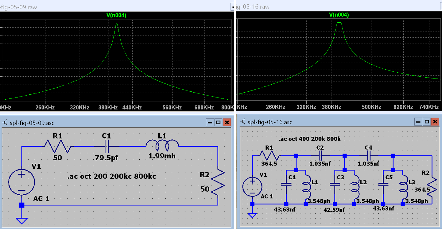
Figure 5.15 Comparing two Different Band Pass Filters.

A professor who is teaching a course in radio receiver design presents figure 5.15 to his students and asks the following question. "Compare and contrast the two filter circuits, point out the advantages and disadvantages of each when used as the intermediate frequency filter in an amplitude modulation radio receiver." The question is printed at the top of a page and the rest of the page is blank. If you were a student in this class how would you answer the question?

This is a trick question. Note that the vertical scales which are attenuation in dB have been cropped out of the picture. The students should answer the question based on the schematic diagrams rather than the frequency graphs. The circuit on the left has only one tuned circuit while the one on the right has 3. The purpose of the IF filter is to pass the wanted signal and attenuate signals on nearby channels. When it comes to receiving the wanted channel and not hearing the adjacent channels, number of tuned circuits is what it's all about. A student who is doing well in the class would know this. One who is not doing so well would likely answer something like this.

The filter on the left is obviously superior to the one on the right. The passband is narrower and has steeper sides. The out of band attenuation is symmetrical and larger than the one on the right.

The answering student made an assumption that both graphs had the same vertical scale. This is not true. Below are the same two graphs but with the scales showing this time and minus the schematic. Not only that, they have been set to be the same. Also cursors are showing on the graphs to provide information about the actual bandwidth of the filter. In receiver design the bandwidth is defined in terms of the -6 dB points rather than the audio standard of -3 dB points. The attenuation from the generator to the output load resistor is 6 dB so the bandwidth limits are taken at -12 dB.

Figure 5.16 Comparing the same two Band Pass Filters but with equal scales this time.

What say you now? The out of band attenuation of the single tuned circuit filter is revealed by the cursers to be -43.5 dB at both 200 and 800 kHz. The stop band is symmetrical but that's the only good thing that can be said about this filter. Although the readout box states "ratio" the frequency at the bottom is the difference not the ratio. This is good because we are given the bandwidth without having to reach for our calculators. It seems as if the folks at LT were a little careless with their labeling. We must admit that the wonderful job they have done in developing this tool means they can be forgiven for a few oversights. And the price is right too.

The point of the above is not to teach band pass filters but to make the point about jumping to conclusions based on incomplete data. LTspice is just another tool. Like any tool if you misuse it, there are likely to be consequences. The good thing is you can't burn your hand or lose a finger by misusing LTspice but you should always remember that it will never replace a breadboard and prototype. Always keep that in mind as you have fun with simulated tubes.

DON'T FORGET TO SAVE THE DRAWING.

If you can honestly checkoff each item on the list under the heading "What you will learn in lesson 5", you can go on to lesson 6, assuming I have written it by then.

Back To Table of Contents.

This page last updated Friday, May 06, 2022.

Home.