
Lab #2 Steady-State One-Dimensional Conduction
With no Source and Boundary
Convection
Problem Statement: Using the Lab02 Matlab Script File for steady-state one-dimensional conduction with no source and boundary convection, perform a mesh convergence study for linear, quadratic, and cubic element bases. Starting with a two element discretization, uniformly refine the mesh 6 times. Verify the asymptotic error estimate using the energy semi-norm and in TL, presenting appropriate tables and graphs.
Analysis:
The following tables were filled out using the equations below:
Note: The user inputs the number of nodes over the domain and Matlab provides the Enorm values and Q at the left most node.
Equations Used
to Fill out Charts
|
Convergence Tables (Linear, Quadratic, Cubic) |
|||||||||
|
Linear Table |
|||||||||
|
Meshelements |
le |
QL |
DQL |
eh/N |
SlopeQ |
Enorm |
DEnorm |
eh/NEnorm |
SlopeEnorm |
|
2 |
0.5 |
996.8656 |
--- |
--- |
--- |
13409102.75 |
--- |
--- |
--- |
|
4 |
0.25 |
999.191 |
2.3254 |
0.7751 |
--- |
13451119.25 |
42016.51 |
14005.5008 |
--- |
|
8 |
0.125 |
999.796 |
0.605 |
0.2017 |
1.942 |
13462049.76 |
10930.51 |
3643.5027 |
1.943 |
|
16 |
0.0625 |
999.9489 |
0.1529 |
0.0513 |
1.978 |
13464812.3 |
2762.54 |
920.8471 |
1.984 |
|
32 |
0.0313 |
999.9872 |
0.0383 |
0.0128 |
1.997 |
13465504.87 |
692.56 |
230.856 |
1.996 |
|
64 |
0.0156 |
999.9968 |
0.0096 |
0.0032 |
1.997 |
13465678.13 |
173.27 |
57.7546 |
1.999 |
|
128 |
0.0078 |
999.9992 |
0.0024 |
0.0008 |
2 |
13465721.46 |
43.32 |
14.4412 |
2 |
|
|
|
|
|||||||
|
Quadratic Table |
|||||||||
|
Meshelements |
le |
QL |
DQL |
eh/N |
SlopeQ |
Enorm |
DEnorm |
eh/NEnorm |
SlopeEnorm |
|
2 |
0.5 |
999.9704 |
--- |
--- |
--- |
13465201.74 |
--- |
--- |
--- |
|
4 |
0.25 |
999.998 |
2.76E-02 |
1.18E-03 |
--- |
13465698.89 |
497.1535 |
165.7178 |
--- |
|
8 |
0.125 |
999.9999 |
1.87E-03 |
1.25E-04 |
3.2495 |
13465733.52 |
34.6273 |
11.5424 |
3.8437 |
|
16 |
0.0625 |
1000 |
1.24E-04 |
8.24E-06 |
3.9174 |
13465735.75 |
2.2323 |
0.7441 |
3.955 |
|
32 |
0.0313 |
1000 |
7.78E-06 |
5.19E-07 |
3.989 |
13465735.89 |
0.1406 |
0.0469 |
3.988 |
|
64 |
0.0156 |
1000 |
4.87E-07 |
3.25E-08 |
3.9976 |
13465735.9 |
0.0088 |
0.0029 |
3.9973 |
|
128 |
0.0078 |
1000 |
-2.95E-08 |
1.87E-09 |
4.0441 |
13465735.9 |
0.0006 |
0.0001 |
4.009 |
|
|
|
|
|||||||
|
Cubic Table |
|||||||||
|
Meshelements |
le |
QL |
DQL |
eh/N |
SlopeQ |
Enorm |
DEnorm |
eh/NEnorm |
SlopeEnorm |
|
2 |
0.5 |
999.9997 |
--- |
--- |
--- |
13465730.72 |
--- |
--- |
--- |
|
4 |
0.25 |
1000 |
2.82E-04 |
4.47E-06 |
--- |
13465735.81 |
5.0867 |
1.6956 |
--- |
|
8 |
0.125 |
1000 |
3.58E-06 |
5.68E-08 |
6.3 |
13465735.91 |
0.1044 |
0.0348 |
5.606 |
|
16 |
0.0625 |
1000 |
-3.79E-06 |
6.01E-08 |
-0.082 |
13465735.94 |
0.0277 |
0.0092 |
1.915 |
|
32 |
0.0313 |
1000 |
-1.48E-05 |
2.35E-07 |
-1.965 |
13465736.04 |
0.1042 |
0.0347 |
-1.913 |
|
64 |
0.0156 |
1000 |
-5.92E-05 |
9.39E-07 |
-2.001 |
13465736.46 |
0.4168 |
0.1389 |
-2 |
|
128 |
0.0078 |
1000 |
-2.37E-04 |
3.75E-06 |
-1.999 |
13465738.13 |
1.6671 |
0.5557 |
-2 |
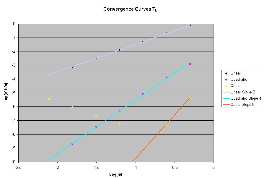
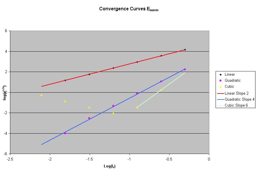
Conclusion:
From the Convergence Curve Graphs
below you can see that the linear and quadratic meshes are within the adequate
mesh zone. The slope of the convergence
curves for these two trials is close to 2 and 4 respectively. Increasing refinement helped the accuracy
for the linear and quadratic trials, however the cubic behaved a little bit
different. As you increased the
refinement on the mesh for the cubic the slope became negative and the curves
became non-linear. This phenomenon is
called “round off error”.
