Two-Way Between-Subjects Analysis of Variance (Chapter 17)
- ONE IV and ONE DV
When we include another IV in our design, we can look at the independent effects of each of the two IVs on the DV as well as the interaction between them
- This is a two-way ANOVA because we’re looking at the joint effects of two IVs on the DV
Factorial Designs
- We test research questions like the one above using Factorial Designs.
- IVs are typically called Factors in two-way analysis of variance.
IV1: Randomly assign people into the None, Mod, and High caffeine groups.
IV2: Ask them if they regularly drink caffeinated drinks (if yes, they’d have a tolerance built up for caffeine).
- This information would allow us to place people into one of the "cells" or conditions
- This is a two-way BS Factorial Design – There are two IVs, each person is placed in only one cell, and each level of one IV is "crossed" with each level of the other IV.
- Crossed meaning that given our levels of the two IVs, we have all possible combinations of levels.
- Specifically, this is a 3 X 2 Factorial Design – 3 levels of IV1 and 2 levels of IV2.
- The number of groups in a factorial design is simply the product of the number of levels of each factor. (e.g., in our 3 X 2 design, we’d have 6 groups).
Use of Two-Way Between-Subjects ANOVA
- The IVs are both between-subjects in nature.
- The IVs both have two or more levels.
- The IVs are combined to form a factorial design.
- The DV is quantitative in nature and measured on a level that at least approximates interval characteristics.
The Concepts of Main Effects and Interactions
- Factorial designs allow us to address three issues.
1. Does the amount of caffeine alone influence anagram performance? (this is what we tested with the one-way BS ANOVA)
- If yes, this is called a Main Effect of caffeine.
- this indicates the effect of caffeine on performance collapsed across, or disregarding, caffeine tolerance.
2. Does tolerance for caffeine alone influence anagram performance?
- If yes, this is called a Main Effect of tolerance for caffeine.
- This indicates the effect of caffeine tolerance on performance collapsed across, or disregarding, the level of caffeine.
3. Do the amount of caffeine and tolerance for caffeine interact in their influence on anagram performance?
(H0: Effect of caffeine is the same for people with tolerance and people with no tolerance)
- If yes, this is called an Interaction Effect
- This refers to the comparison of cell means in terms of whether the nature of the relationship between one of the IVs and the DV differs as a function of the other IV.
- What’s an interaction effect?
- A joint influence of multiple IVs
- The effects of one IV depend on the other IV
- One IV changes the relationship between the other IV and the DV
Identifying Main Effects and Interactions
- How do we test for main effects and interaction effects? - ANOVA – we partition variability in our DV scores into components that allow for testing each Main Effect and the Interaction Effect.
- Statistically speaking, a main effect is present if we reject the null hypothesis of no main effect.
- Similarly, an interaction is present if we reject the null hypothesis of no interaction.
- Conceptually, we can take a different approach:
- For our Main Effects, we’d be testing for statistically significant differences among the Marginal Means (collapsed across the other IV)
1. Main effect for amount of caffeine
- testing for differences among the marginal means 69, 82, 62
2. Main effect for tolerance for caffeine
- testing for differences among the marginal means 64 and 78
- (We would need our significance tests to determine if the main effects were statistically significant.)
- For the Interaction Effect, we’d test for certain patterns of differences among the Cell Means
- Does the effect of amount of caffeine on anagram performance change as a function of tolerance for caffeine?
- This is easiest to conceptualize by graphing the means
- If the lines cross, or at least are not parallel, this suggests a potential interaction effect.
- (We would need our significance test to determine if the interaction is statistically significant.)
Inference of Relationships Using Two-Way Between-Subjects ANOVA
Partitioning of Variability
- Recall in the BS ANOVA we partitioned the total variability of the DV.
![]()
- The quantities ![]() and
and ![]() were divided by their respective degrees of freedom to obtain
were divided by their respective degrees of freedom to obtain ![]() and
and ![]()
- An F ratio was then formed by dividing![]() by
by ![]() .
.
- The ![]() in two-way ANOVA can be similarly partitioned into
in two-way ANOVA can be similarly partitioned into ![]() and
and ![]()
- However, the overall sum of squares between is further partitioned into three components:
1. Variability due to the first IV (e.g., level of caffeine)
2. Variability due to the second IV (e.g., tolerance for caffeine)
3. Variability due to the interaction of the two IVs (level X tolerance)
![]()
- Thus, the total sum of squares can be represented as:
![]()
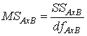
- In two-way ANOVA, each of the components of the sum of squares between is divided by its respective degrees of freedom, and the resulting mean squares (![]() , (
, (![]() ), and (
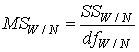
), and (![]() ) are then divided by the (
) are then divided by the (![]() ) to yield F ratios.
) to yield F ratios.
Derivation of the Summary Table
|
Source |
SS |
df |
MS |
F |
|
A (Caffeine) |
SSA |
dfA= (a - 1) |
|
|
|
B (Tolerance) |
SSB |
dfB= (b - 1) |
|
|
|
A X B (interaction) |
SSAXB |
dfAXB= (a-1)(b - 1) |
|
|
|
Within Cells |
SSW/N |
dfW/N= (a)(b) (n - 1) |
|
|
|
Total |
SSTOT |
dfTOT= (N - 1) |
|
|
Inference of Relationships
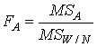
- The test of the null hypothesis for the main effect of level of caffeine is made with reference to the F value derived from ![]()
- This value is compared against the critical value corresponding to the appropriate degrees of freedom.
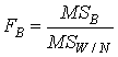
- The test of the null hypothesis for the main effect of tolerance for caffeine is made with reference to the F value derived from ![]()
- This value is compared against the critical value corresponding to the appropriate degrees of freedom.
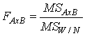
- The test of null hypothesis for the interaction effect is made with reference to the F value derived from ![]()
- This value is compared against the critical value corresponding to the appropriate degrees of freedom.
Strength of the Relationship
- The strength of the relationship between the dependent and each of the sources of between-group variability is computed using the following formulas for eta-squared.
![]()
![]()
![]()
Nature of the Relationship
Analysis of Main Effects
- When a statistically significant main effect has only two levels, the nature of the relationship is determined in the same fashion as for the independent groups t test.
- Which mean is higher/lower than the other?
- When a statistically significant main effect has more than two levels, the nature of the relationship is determined using a Tukey HSD test conceptually identical to the one used in the one-way ANOVA.
![]()
Analysis of Interactions
- When an interaction effect is statistically significant, the nature of the interaction can be determined using a number of statistical procedures.
- One popular procedure is the use of an analytic method called simple main effect analysis.
- A second approach is called interaction comparisons.
Methodological Considerations
- When we covered the caffeine example in Chapter 12, we discussed that caffeine tolerance could be a disturbance variable, increasing the within group variability.
- Now, we have combined caffeine tolerance with level of caffeine to create 6 groups, and the within-group variability is based on the variability of scores within each of the 6 groups separately.
- Not only do they allow us to assess the interaction between independent variables, but they also "remove" the individual and joint effects of these variables from the within-group variability.
- This makes the tests of the main effects more sensitive than if one of the variables was left uncontrolled and took on the role of a disturbance variable.