The kind of significant difference test we do depends on our situation. There are several kinds; they are as follows:

1) One-sample significant difference tests are done to evaluate the difference between a single sample and a population. They are the subject of this chapter.

2) Two-sample significant difference tests are done to evaluate the difference between two samples. They will be discussed in Chapter 7.

3) Analysis of variance (ANOVA) is done to evaluate differences among 3 or more samples. While these tests are described in Chapter 8, they are beyond the scope of this course and will not be further discussed.

4) Factorial analysis of variance is used when two or more independent variables are being evaluated. Chapter 9 includes discussion of these techniques; however they will not be discussed in this course.

Significant difference tests can be categorized another way, as parametric or nonparametric. Parametric tests are based on specific assumptions about the data being analyzed, so they can be used only when these assumptions are accurate. The parameters or characteristics the data are assumed to have are generally that the data are continuous, that the variable under study is normally distributed in the population, and that variances are similar in samples being compared. When we look at specific tests, we’ll discuss their particular assumptions.

If your data violate the assumptions of the parametric tests available, then nonparametric tests must be substituted. As a rule, nonparametric tests have less statistical power (ability to detect significance) than their parametric alternatives, so where possible the parametric tests are preferred.

One-sample significant difference tests tell us whether the difference between a sample and a population is statistically significant. They are used in two kinds of situations.

The first is to evaluate the representativeness of a sample. Here’s the problem: when you draw a sample from a population for study, you intend to take what you discover from the sample and generalize it to the whole population. This is a good idea only if the sample accurately reflects the characteristics of the population; otherwise your assumptions about the population based on the sample could be faulty. A sample that accurately reflects the characteristics of the population is said to be a representative sample—it represents the population accurately.

Now we know that any sample we draw from a population is likely to be somewhat different from the population; the question is whether the sample is sufficiently different to make using it questionable. A sample which is only a little different would be OK to use; one that is very different would not be OK to use. The problem is how to know which is which. When evaluating the representativeness of a sample, we hope to find that the sample is not significantly different from the population from which it was drawn. This would mean that it accurately represents the population and is just fine to study.

Let’s look at an example:

Suppose you were interested in studying obesity in Presentation College students. Let’s say you’re measuring body-mass index (BMI), a computed measure of weight for height, and you decide to draw a sample of 20 students. Now you know it’s quite likely that any sample you draw will have a different average BMI from the entire student population, simply due to sampling error. That’s the way it goes when you’re studying samples. You’d simply accept this difference and proceed with your study.

Now suppose you decide to select your sample of students by hanging around the Strode Center on a winter afternoon, selecting the first 20 students you see. Well, you’d likely end up in the middle of basketball practice, selecting 20 athletes. Will this sample differ from the population? Almost certainly. Will the difference in BMI be purely due to sampling error? I doubt it! My guess is that the athletes will have lower BMIs than the general run of students because they’re in pretty good physical condition compared to everyone else. This is a sample that is different from the population in an important way that goes well beyond the effects of sampling error. This is a difference we wouldn’t want to just accept and go on because it would cause us to draw faulty conclusions about our population; the sample doesn’t accurately represent the general student population.

The trick is how to tell the difference. Supposing you don’t make such an obvious error in sampling (which someone will be happy to point out to you), you’ll need some means to determine whether the differences you see are due to sampling error or to something else. That’s what significant difference testing is all about.

So when you want to know whether your sample is appropriate for generalizing to the population, a significant difference test that shows no significant difference between your sample and the population will tell you that you have a representative (appropriate) sample.

The other situation in which we might use a one-sample significant difference test is when we want to evaluate the effect of some independent variable on a characteristic of the sample. Let’s say we’re interested in the effect of sun exposure on skin redness. (This is Chapter 1; do you remember? Sun exposure is the independent variable; skin redness is the dependent variable.) We call the independent variable a treatment and the effect of the independent variable a treatment effect. In this case, the treatment effect is increased redness of the skin. What we’d do in our study is draw a sample and expose these cases to the sun. Then we’d compare the skin redness of the sun-exposed sample to the skin redness of the population. What we’re interested in here is whether the sample has significantly more skin redness than the population—a treatment effect. So we’d subject our skin redness measurements to a one-sample significant difference test.

If the sample has significantly more skin redness than the population, then we’d conclude that there was a treatment effect. If the sample does not have significantly more skin redness than the population, then we’d conclude that there was no treatment effect.

Note that we can use the term treatment fairly loosely here. A treatment does not have to be something we deliberately control or manipulate in an experiment as we did the sun exposure. Let’s say we were studying the effects of high fat diets on rates of heart disease. We might find a group of people with unusually high-fat diets and compare their rates of heart disease with those in the population. Here the treatment is the high-fat diet, even though we didn’t actually administer the treatment ourselves; the subjects of study did that without our help even before we began to study them. The treatment effect we’re looking for is an increased rate of heart disease.

And in our example of the BMI study where we selected our sample from the basketball team, the difference we see in BMI among our sample is also a treatment effect. Their lower BMI reflects a true difference from the population—probably one that is statistically significant—so we would call it a treatment effect. The treatment is that these students in the sample are all athletes, even though you, the researcher, did not control or administer this treatment.

Now things should begin to make sense. We know that almost any sample will differ from its population; this is an old idea we’ve talked about before. A significant difference is a reliable one, one that reflects an actual difference between the sample and a population, not just the effect of sampling error. What we need is a way to sort out small differences which are due to sampling error from those slightly bigger ones which are due to a treatment effect. We need a place to draw the line between significant and nonsignificant differences; the way we find that place is the significant difference test. Doing this job enables us to accomplish two kinds of things. One is to evaluate the representativeness of a sample to determine whether it is like enough to the population so that we can rely on sample results to draw conclusions about the population. The other is to evaluate a treatment to see whether it had an appreciable (significant) effect on the sample.

Whenever we compare a sample and the population from which it is drawn, we know there will almost certainly be a difference; the significant difference test is to figure out what this difference means. Basically, there are two possible explanations for difference between a sample and the population; we can write two hypotheses to cover these explanations.

One explanation for a difference between a sample and the population is that the difference is due simply to sampling error. This explanation, the Null Hypothesis, explains away the observed difference by saying it is small enough to be expected in a sample drawn from that population, and that other samples drawn from the population would likely show similar size differences. This means that the sample is really very like the population; there is no treatment effect operating here. The hypothesis says that the sample accurately reflects the characteristics of the population and that the difference observed between the sample and the population is statistically non-significant.

So what would we write for a null hypothesis? Let's think about the study of the effects of sun exposure on skin redness. Remember that the null hypothesis is one of the two possible explanations for the differences seen. How about this?

H₀ (the Null Hypothesis): The difference between the mean skin redness of the sample and that of the population is no greater than would be expected due to sampling error. There is no treatment effect operating here; so the difference is nonsignificant. Sun exposure does not cause increased skin redness.

The other explanation for a difference between a sample and the population is that the difference observed is the result of the sample being treated differently from the population in some way. This explanation, the Alternative Hypothesis, declares that the observed difference is too great to attribute to sampling error. This means that the sample is not like the population, but shows treatment effect. The hypothesis says that the sample does not accurately reflect the characteristics of the population; it is, in fact, different from the population in some important way, and the difference observed between the sample and the population is statistically significant.

H₁ (the Alternative Hypothesis): The difference between the mean skin redness of the sample and that of the population is too great to attribute to sampling error. It is due to treatment effect; so the difference is significant. Sun exposure does cause increased skin redness.

Because these are two mutually exclusive explanations for difference, when you’ve performed a significant difference test, you will be able to accept one of these hypotheses and reject the other. So if your test tells you that the difference is statistically non-significant, then you’ll accept H₀ and reject H₁. This means that your explanation for the difference you observed is that it is due to sampling error—no big deal, not significant, no treatment effect observed. On the other hand, if your test tells you that the difference is statistically significant, then you’ll accept H₁ and reject H₀. This means that your explanation for the difference is treatment effect—significant, not just sampling error. Always, your results from your significant difference test will enable you to accept one hypothesis and reject the other--can't accept both.

So there are three parts to a good hypothesis:

1. The difference you're seeking to explain must be stated explicitly, for example, the difference between the mean skin redness of the sample and that of the population.

2. The explanation for the difference. Either the difference is small enough to attribute to sampling error and is nonsignificant, or the difference is too big to attribute to sampling error and is due to treatment effect.

3. A sentence that puts your findings in terms of the study at hand. That means that you must interpret the significance or nonsignificance of the result according to what it means in the study you're doing. Here is where you tell what conclusions you draw as a result of your findings.

THE ONE-SAMPLE t TEST

The t test is used to evaluate differences between the sample mean and the population mean. It is a parametric test, which means the test is valid only if the data being analyzed conform to the assumptions of the test. These parameters for the one-sample t test are that the data must be continuous and that the characteristic being measured must be normally distributed in the population. The more important of these parameters is the one requiring continuous data. As long as sample sizes are large enough (You guessed it—at least 50.), then violations of the assumption about normal distribution are not a big deal. So, with all sample sizes, the data need to be continuous; and for small sample sizes, the population distribution for the characteristic measured needs to be normal.

Our determination of just how big a difference has to be in order to be significant can be influenced a lot by the kinds of numbers we’re measuring. Let’s say we’re studying the mean number of children per family. The population mean might be 2.40, so a sample mean of 5.00 (difference of 2.60 children) is probably going to turn out to be significant. On the other hand, if we’re studying mean annual income, the population mean might be $21,500, and a difference of 2.60 dollars would almost certainly mean nothing at all. So any test that simply established an absolute size difference that would be significant would probably lead to all kinds of wrong conclusions.

What we need to do is to find a way to standardize the size of the difference seen between the mean of the sample and the mean of the population, no matter how big or small our means. That way we get a number we can interpret no matter what we’re measuring. The way we do this is to use a test statistic, a number that varies as the size of the difference varies, but in terms of some standard yardstick. The test statistic we use is called t, and it puts the difference of means in terms of the number of standard errors of the mean involved. What t tells us is how many standard errors wide the difference of means is. Here’s how we obtain a value for t using our data:

What you’re doing is taking the difference in means in actual units measured (number of children, dollars of income, inches of length, or whatever) and reporting it in terms of standard errors. So the t statistic tells us how many standard errors the difference is, instead of how many children, dollars, etc. This gives us a standardized number we can interpret in the same way, no matter what our original units of measurement were. And you already know how to figure out the standard error of the mean, so finding the obtained t shouldn’t be difficult. Do remember all the ways there are to get into trouble when computing standard error—correcting the variance, forgetting whether variance or standard deviation is needed, computational error.

Now that you have a number for your test statistic, obtained t, what comes next? You need to evaluate the standardized difference in means (t) to decide whether the difference is big enough to be significant.

The Sampling Distribution of t: For that, we go to a method much like the one you used in Chapter 5. We can make a sampling distribution of t by drawing all possible samples of size N from the population, computing t for each sample, then making a frequency distribution of the resulting values of t. This is almost like a sampling distribution of the mean; the only difference is that we’re computing t for each sample instead of computing the mean for each sample.

Like all sampling distributions, the central limit theorem applies: the population mean equals the mean of the sampling distribution. Since the mean t score is 0 (a difference of no standard errors), then the center of the sampling distribution occurs at 0, with negative values of t to the left and positive values of t to the right.

Also according to the central limit theorem, if sample sizes are large enough (at least 50), the sampling distribution is normal in shape. When samples are smaller, then the shape of the sampling distribution depends on the shape of the distribution in the original population. A pretty normal population distribution with small samples gives a more-or-less normal, but flattened, sampling distribution—and the amount of flattening is predictable for a particular sample size. A nonnormal population distribution with small samples gives you a mess. Since this mess is too complicated to figure out, one of the parameters of the t test is a normal-shaped population distribution when samples are small. What we’re doing here is eliminating the mess by insisting on using the t test only when the population distribution is normal or sample sizes are big.

Because the shape of the sampling distribution is fairly predictable as long as the population distribution is normal, it is possible, using calculus, to figure out the shape this sampling distribution will have for various sample sizes. It is also possible to mark off various areas under the curve (90%, 95%, etc.) and figure out the values of t that occur at our marks.

Here’s why we care: the sampling distribution of t shows all the possible values of t you can get purely due to sampling error. (This is the same story as we had with the sampling distribution of the mean; it showed all the sample means you can get purely due to sampling error.) This gives us a picture of how big differences are likely to be if they’re due just to sampling error, not to treatment effect; and that can serve as a sort of standard against which we can measure our difference to see how it stacks up.

We can look at significance in just the same way as we did in Chapter 5. If our value of t (which reflects a specific difference between sample and population mean) falls within the area encompassing the 95% of the area around the mean value of t, then we can conclude that it is 95% likely to be due to sampling error, not to treatment effect.

One-Tail Tests: Now we do have a new wrinkle in this whole thing that we didn’t have to consider in Chapter 5. Sometimes when we’re looking for treatment effect, we expect the sample mean to differ from the population mean in a specific direction. For example, in the study of the effects of sun exposure on skin redness, we expect sun exposure to produce increased redness. So we don’t expect a decrease in redness, and we’re really only able to say the sun changes skin redness if the skin gets MORE red. When we’re able to predict a direction of difference (predicting that the sample mean will be greater than the population mean OR that the sample mean will be smaller than the population mean), we use what is called a one-tail test. That means that we’re only interested in one of the two tails we see on a frequency distribution. A significant difference will show up only in one of the tails—which one depends on the direction of difference we’ve predicted. To show the situation for our sun exposure study, I’ve constructed the following graph:

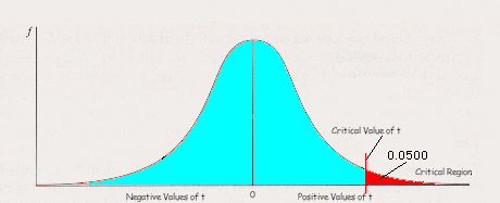
What we’ve done here is construct the sampling distribution of t for our particular sample size, showing the mean value of t as 0 and indicating that positive values of t occur to the right of the mean and negative values of t occur to the left of the mean. Then we’ve marked off 95% of the values, leaving 5% all in the right-hand tail, where we’d find values indicating the sample mean is greater than the population mean. This is because we’ve predicted increased skin redness in the sample, so redness values for the sample will be higher than those in the population if sun does indeed increase skin redness.

We call the red 5% a critical region. The critical region contains values of t which have a less than 5% probability of occurring due to sampling error, so values which occur in the critical region are said to be significant at the 0.05 significance level. (We write this as p<.05.) The value of t which marks off this critical region is the critical value of t, and is included in the critical region. This means an obtained t exactly equal to the critical value of t would be considered IN the critical region.

Now you see how we can interpret our obtained t to decide whether the difference we’ve observed between our sample and our population means is significant. If the obtained t falls in the critical region for our sample size, then the difference is statistically significant (accept H₁ and reject H₀); if it is outside the critical region (in the turquoise 95% area), then the difference is nonsignificant (accept H₀ and reject H₁).

Two-tail Tests: Now sometimes we don’t have enough information to predict a direction of difference. We just want to know whether the sample mean is significantly different from the population mean; and a difference in either direction would interest us. In this case, we’re interested in both tails of the sampling distribution, so our 95% would have to come out of the middle of the distribution, leaving 2.5% in each tail for 2 critical regions.

Once again, the critical values of t mark the beginning of the critical regions and are included in the critical regions. The critical regions contain values which have only a 5% probability of occurring due to sampling error. So when the obtained t falls in a critical region for our sample size, then we declare the difference to be statistically significant (accept H₁ and reject H₀); if it is outside both critical regions (in the turquoise 95% area), then we call the difference nonsignificant (accept H₀ and reject H₁). Here’s the picture:

Critical Values of t: Now the only thing left to do is figure out how we find the critical value for t that marks the beginning of the critical region(s) in either the one-tail or two-tail t test. It is fortunate that a friendly math expert has worked out the details using a bit of calculus (and a computer). And for our convenience a bunch of relevant values are listed on a table called Critical Values of t, which can be found in Appendix B of your textbook on page 403.

Take a look at the t table. This should be just a refresher since you used this table to do interval estimation in Chapter 5. Down the left side of the table are values listed from 1 to 30, then a few others up to infinity. The heading on this column is df, which you already know means degrees of freedom. (What this means is the number of values in a sample which are free to vary while still averaging up to the sample mean; don’t worry too much about this definition.) For the one-sample t test, this number will always be N – 1. Remember that the sampling distribution of t will change shape as N changes, so this is how you account for your sample size when finding critical values of t. Then across the top of the table are two sets of column headings; one is labeled Level of Significance for One-Tail Test, and the other is labeled Level of Significance for Two-Tail Test. The values listed in these columns are the values for t that mark off the critical regions for different sample sizes at various levels of significance.

So you need three pieces of information to enter the t table to find a critical value of t. These are the sample size (from which you can derive the degrees of freedom), whether you’re doing a one-tail or a two-tail test (which you decide based on whether you were able to predict a direction of difference between the sample and population means), and the significance level (which you learned to figure out doing interval estimation in Chapter 5).

Sample Problem #1: Let’s do an example based on your sun exposure and skin redness study. Say your sample size is 25 and we’re interested in the 0.05 significance level. The mean redness (on a scale of 1 to 10) in the population is 2.5. The mean redness in the sun-exposed sample is 3.88, with a standard deviation of 2.08.

OK, so we have a difference in skin redness between our sample and our population. There are two possible explanations for this difference. They were stated earlier; here they are:

H₀ (the Null Hypothesis): The difference between the mean skin redness of the sample and that of the population is no greater than would be expected due to sampling error. There is no treatment effect operating here; so the difference is nonsignificant. Sun exposure does not cause increased skin redness.

H₁ (the Alternative Hypothesis): The difference between the mean skin redness of the sample and that of the population is too great to attribute to sampling error. It is due to treatment effect; so the difference is significant. Sun exposure does cause increased skin redness.

In order to test these hypotheses, we need to obtain a value for t and determine whether this value falls into the critical region on the sampling distribution of t. This will enable us to decide whether the difference between the means is significant. To compute t, we need the corrected standard error of the mean; and to compute this, we need a corrected standard deviation. So let’s start:

We already decided this study would use a one-tail test since we predicted a direction of difference—that the sun-exposed sample would show increased skin redness. So what is your critical value of t? You’ll read the row for df = 24 (N – 1); under one-tail tests, you’ll read the column for 0.05 level of significance. Moving to where this row and column intersect, you find a value of 1.711. This is the critical value of t, the value that marks off the beginning of the 5% critical region in the right-hand tail of a sampling distribution when N = 25. When you’re interpreting the result of a significant difference test on this sample, you’ll compare your obtained t to the critical value for t. If your obtained t is in the critical region marked off in the right-hand tail by t = 1.711, then the difference you found is significant at the 0.05 level. This means that an obtained value of t which is 1.711 or greater indicates a significant difference between the sample and the population means. If your obtained t is not in the critical region, then the difference you found is nonsignificant at the 0.05 level. This means that an obtained t which is less than 1.711 indicates the difference between the sample and population means is nonsignificant. In this example our obtained t is 3.255, a value greater than 1.711, so the difference is significant.

Now, back to our 2 hypotheses. H₀ attributes the difference in means to sampling error, concluding that the difference is not significant. Since this hypothesis doesn’t fit with our results, we reject H₀. That means we accept H₁, which claims that the difference is due to treatment effect and is significant. This hypothesis fits very well with our results. We can, therefore, conclude that sun exposure does indeed cause increased skin redness.

Sample Problem #2: Now let’s suppose you’re doing a study of a new sunburn cream which is claimed to reduce skin redness within 1 hour of application. One way to test this cream is to take a population of sunburned people and measure their skin redness. Then select a sample (N = 25) and apply the cream; wait one hour; and measure their skin redness.

Here are your measurements: mean skin redness in the population is 3.88; mean skin redness in the sample is 3.25, with a standard deviation of 1.91. We need two hypotheses:

H₀: The difference between the mean skin redness of the sample and that of the population is no greater than would be expected due to sampling error. There is no treatment effect operating here; so the difference is nonsignificant. The cream does not reduce skin redness.

H₁: The difference between the mean skin redness of the sample and that of the population is too great to attribute to sampling error. It is due to treatment effect; so the difference is significant. The cream does reduce skin redness.

Let’s do the math:

Now we have a negative value for the obtained t. What do we do with this? The first thing to do is to remember the characteristics of the sampling distribution of t: it is symmetrical with 0 at the mean, positive values to the right of the mean, and negative values to the left of the mean. That means that the value, -1.615, is just as far to the left of the mean as the value, +1.615, is to the right of the mean. So we can place our obtained t on the sampling distribution.

Now, once again, we’re doing a one-tail test because we’ve predicted a direction of difference. We are looking for the cream to reduce skin redness, so this time the tail we’re interested in is the one on the left. When we look up a critical value of t, we’ll want the negative value to mark off the critical region. (This works much like looking up both positive and negative z-scores in the same place in the Table of Areas.) So, whatever value of t we settle on for a critical value, we’ll use the negative of that value and place it to the left of the mean on the sampling distribution. So here goes: one-tail test, df = 24, 0.05. The value we find on the chart is 1.711; our critical value of t (which is a negative number this time) is –1.711.

This time, since –1.711 marks the start of the critical region, a significant obtained t will be –1.711 or less (more negative). So, -2.000 would be significant, but –1.500 wouldn’t. Our obtained t is –1.615—outside the critical region. So the difference is nonsignificant.

As for our hypotheses, H₀ attributes the difference in means to sampling error, concluding that the difference is not significant. Since this hypothesis fits with our results, we accept H₀. That means we reject H₁, which claims that the difference is due to treatment effect and is significant. This hypothesis doesn’t fit with our results. We can, therefore, conclude that the cream does not reduce skin redness; it doesn’t live up to the manufacturer’s claim.

Sample Problem #3: Now let’s take a look at the BMI study for which we drew a sample of PC students a while ago. Now let’s say we’ve drawn a sample of 20 students for the obesity (BMI) study and we want to check the sample to see whether it is representative of the student population. Remember that the 0.05 significance level is sort of standard, so when no significance level is given, this is the one you should use.

The mean BMI for our population is 25.2 (which is a little high); for our sample it is 22.4, with a standard deviation of 3.8. Let’s see whether this difference is means is significant. Of course, first we need to write our two hypotheses:

H₀: The difference between the BMI of the sample and that of the population is no greater than would be expected due to sampling error. There is no treatment effect operating here; so the difference is nonsignificant. The sample is representative of the population.

H₁: The difference between the BMI of the sample and that of the population is too great to attribute to sampling error. It is due to treatment effect; so the difference is significant. The sample is not representative of the population.

Now we can do the math:

Now we need to look up the critical value for t you’ll use in this significant difference test. When you’re checking to see whether a sample is representative, you’re interested in differences in either direction, so you should be doing a two-tail test. You’re using the 0.05 significance level and df = 19. The critical value of t is 2.093. Now since this value marks off two tails, we must use +2.093 to mark off the right-hand tail and –2.093 to mark off the left-hand tail. So if your obtained t is in either of the critical regions marked off by these two critical values of t, then the difference between the sample and the population is significant. If the obtained t is not in either critical region (but in the middle 95%), then the difference between the sample and the population is nonsignificant. Your obtained t is –3.218—way out in the critical region on the left side of the sampling distribution, so the difference between sample and population means is significant.

This makes it easy to choose a hypothesis. H₀ attributes the difference in means to sampling error, concluding that the difference is not significant. Since this hypothesis doesn’t fit with our results, we reject H₀. That means we accept H₁, which claims that the difference is due to treatment effect and is significant. This hypothesis does fit with our results. We can, therefore, conclude that our sample is not representative. This would mean the sample is not a good one to study if you want to generalize from your study results to the rest of the students at PC. I guess it was a big mistake to blunder into basketball practice in order to choose a sample.

MOST COMMON MISTAKE: Getting one-tail and two-tail tests mixed up.

SECOND MOST COMMON MISTAKE: Getting confused about just what your results tell you. This can cause you to forget where you left off and declare significance just opposite to the correct way. It will help to avoid this mistake if you write both a Null and an Alternative Hypothesis for every problem, then interpret your significant difference test result according to the 2 hypotheses you have.

ONE OTHER PROBLEM THAT TURNS UP A LOT: Messing up in computing standard error of the mean. Sometimes people forget they need to use a corrected standard deviation; especially when samples are small, this leads to mistakes. Then sometimes, people mix up variance (s²) and standard deviation (s), using the wrong one to get standard error of the mean. Another thing that happens frequently is that people get so immersed in all the calculations when correcting variance and all that they forget to finish and find the standard error of the mean; they just use the corrected standard deviation instead. Watch all of these steps carefully as you perform them.

I am strongly recommending that you do every single practice problem provided in the textbook before tackling the worksheet for this chapter. That will clean up many of your mistakes before you get to the worksheet at all.

There is a nonparametric test to use for one-sample significant difference testing when your data fail to conform to the parameters of the t test. This nonparametric test is the Chi-square goodness of fit test; and it can be done on nominal or continuous scale data. It makes no difference whether the characteristic of interest is normally distributed in the population. There are no prior requirements on the data for performing a Chi-square test. There is a trade-off for this easy-going situation; that is that the Chi-square test is much less powerful than the t test. That means the Chi-square test is much more likely to miss out on identifying significance where it exists. On the other hand, sometimes you have a sample and a population that are quite a bit different, but still happen to have the same mean. Chi-square will detect the differences here that a t test would miss entirely.

Chi square is a test statistic, just as t is. So Chi-square varies with the differences between the groups tested; what we do here is square, standardize, and accumulate differences between expected and observed frequencies in each category of the dependent variable to get the test statistic. Here’s the formula for Chi-square:

Let’s say you’re interested in ages of college freshmen in South Dakota. You know that nationally 63% of college freshmen are 21 and under; 27% are from 22 to 30; 7% are from 31 to 39; and only 3% are 40 or older. These numbers are called population percentages, and they represent the population numbers to which you’ll compare your sample numbers. Let’s put this into a table for easy reference:

Here’s a suggestion: add up the population percentages and make sure they add up to 100%. If they don’t you’re missing a category somewhere; figure it out before you go on.

Suppose your sample consists of 1000 freshmen in South Dakota colleges. Now if your sample were exactly like the national population, what number of this 1000 would be 21 and under? It should be 63% of the 1000, or 630, shouldn’t it? This number (630) is called an expected frequency, the number you’d expect to see in this category if there were no differences between your sample and the population. Then how many of your 1000 would you expect to be from 22 to 30 years old? Should be 27% of 1000 or 270. So 270 is the expected frequency for this age group. Do the expected frequencies for each of the other 2 age groups. Don’t look on until you’ve finished; the answers follow.

For the 31-39 age group, I’d expect to see 7% of the 1000 or 70 in the sample; and for the 40 and older age group, I’d expect to see 3% or 30 in the sample.

The most common mistake in doing Chi-square tests is in this step—finding expected frequencies. It’s good to know that there’s a way to check your work at this point: add up your expected frequencies; they should add up to N, with some allowance for rounding (when your multiplication doesn’t work out to whole numbers). If you add up these numbers and get some number besides 1000, say 728 or 1012, then this is a signal that you’ve made a mistake on the expected frequencies; and you can check you work before you go on.

Now let’s say your actual counts for your sample are as follows: 21 and under—615; 22-30—282; 31-39—78; 40 and over—25. These actual counts are called your observed frequencies; and they should add up to N too; if they don’t, you’ve missed something somewhere.

You’ve probably noticed that the expected and observed frequencies in each category differ. Once again, we can write 2 hypotheses to cover the possible explanations for these differences. Here they are:

H₀: The null hypothesis claims that the differences observed are simply due to sampling error; they are too small to be attributed to treatment effect and are nonsignificant. So the sample is very like the population.

H₁: The alternative hypothesis claims that the differences observed are too great to attribute to sampling error and are therefore due to treatment effect; the differences are significant and the sample is different from the population.

Now what we need to do is find your obtained Chi-square using the formula. Here are the steps: determine the difference between the expected and observed frequencies for each category, square these differences, then standardize by dividing by the expected frequency. The last thing we do is sum the results of this step to get chi-square.

Let’s set this problem up. The easiest way to do chi-square problems is to set up columns to show the steps in computation, just as you did back in Chapter 3 when finding variances. We can use the start we made above when we listed categories for the dependent variable and population percentages. Then we can add columns for the observed frequencies (actual counts in your sample), the expected frequencies (computed above based on sample size), and then the steps in your computation. Here it is with the numbers we have so far:

And now we can do the math and fill out the remaining columns, adding up the final column to give us our obtained Chi-square.

You can see that the computations required to find chi-square simply proceed from left to right until you can sum in the final step. This sum (2.637) is the obtained chi-square.

Now, in order to decide whether the sample is significantly different from the population, we need a critical value for chi-square. This value is derived from a sampling distribution, just as the critical value for t is. The sampling distribution of chi-square is not quite like other sampling distributions because there are no negative values for chi-square. If you look at the formula, this will make sense; you square the differences, which means there are no negative values remaining after this step. As a result, the sampling distribution of chi-square looks like the right side of a sampling distribution; there is a picture in your textbook on page 168. This means all chi-square tests are one-tail because there is only one tail to deal with.

This time, sample size isn’t important to the shape of the sampling distribution. What determines this shape is the number of categories. So degrees of freedom are determined by the number of categories and are defined as df = k – 1, where k is the number of categories. Once again, the hard work has been done for us; and the values of chi-square that mark off various percentages of the area under the distribution for varying numbers of categories have been determined and listed in a table. The table is Table 3, Critical Values of Chi-Square, on page 404 in your textbook.

We enter this table with a specified number of degrees of freedom in the left-hand column and a particular significance level across the top. The intersection of these will give you the critical value of chi-square for your sample. Let’s look up the critical value of chi-square for our example. df = k – 1 = 4 – 1 = 3 and the significance level (if none is specified) is 0.05. Reading from the table, the critical value of chi-square is 7.815.

Once again, this critical value marks the beginning of the critical region; obtained chi-squares that fall within the critical region are significant. Our obtained chi-square is 2.637; it falls outside the critical region. This means our sample does not differ significantly from the population; the differences we see between expected and observed frequencies in the various categories are not statistically significant at the 0.05 level.

When we determine significance in the chi-square test, we accept one hypothesis and reject the other, just as we do with the t test. In the example above, we have accepted H₀ and rejected H₁.

There is a problem with the chi-square test. The test statistic doesn’t work well when the data produce low expected frequencies. The reason for this is that if expected frequencies are very low, a small difference in frequencies can generate a very large obtained chi-square. Think about it: if the expected frequency in just one category is 1 and the observed frequency is 5 (a difference of 4), then the number appearing in the final column for this category is 16. Even before we add in the values for the rest of the categories, we have a huge obtained chi-square.

Because of the effect of low expected frequencies on obtained chi-square, we have some rules to follow. When k =2, then both expected frequencies must be at least 5. When k >2, then no more than 20% of expected frequencies may be less than 5 and no expected frequency may be less than 1.

So what do we do when we have too many small expected frequencies? One possibility is to combine two or more categories that have low expected frequencies so that their combined expected frequency is greater. Another possibility is to work with a larger sample, which will give greater expected frequencies in all categories. Since it is possible to compute expected frequencies for a given sample size before you ever begin a study, you can spot the need for a larger sample before its too late.

Whenever we make decisions based on probability, we know up front there’s some chance we’ll be wrong. Statistics, after all, is built around playing these sorts of odds. While we’d like to be 100% sure all of the time, in fact the less-than-perfect probabilities we use in statistics are often the best—or only—means we have for making the decisions we make. So we try to be honest with ourselves about the chance we’ll be wrong and proceed to use the procedures we have. There are two kinds of statistical decision errors which can occur in significant difference testing. They are called Type I and Type II errors.

Think about the way we decide whether a difference is significant. We look at a sampling distribution for the test statistic. All of the values on the sampling distribution are caused by sampling error. We then mark off some percentage of the sampling distribution, say 95%, and declare any differences that fall within this area to be nonsignificant—that is, due to sampling error. Those outside the 95% area—out in the critical region(s)—we declare too big to be sampling error, so we attribute them to treatment effect.

Think about this. The values in the 5% tail(s) on the sampling distribution ARE due to sampling error; they reflect big differences and are unlikely to occur, but they can occur—that’s how they ended up in the sampling distribution. These values are unlikely to be due to sampling error, but they could be.

Here’s the source of Type I error—falsely calling treatment effect what is really sampling error. In other words, Type I errors result from accepting H₁ when we shouldn’t. Now we know this problem exists; that’s why we say we are only 95% sure. We know we’re likely to be wrong 5% of the time. And the chance of a Type I error occurring is exactly related to the significance level. At 95%, the chance of a Type I error is 5%. We can reduce the chance of a Type I error by increasing our significance level to 99%. Now the chance of making a Type I error is reduced to only 1%. But the chance is still there. There just isn’t a practical way to reduce the probability of making a Type I error to 0 unless we’re willing to call all differences nonsignificant. (In that case, why run the test at all?)

And that brings us to the other kinds of decision error, Type II, where we falsely call sampling error what was really treatment effect. A treatment could produce an effect which is small enough to be a likely result of sampling error alone. Even though it is not really due to sampling error alone, we’re likely to think it is and declare the difference nonsignificant (not due to treatment effect). The fact is that even a small difference might be due to a treatment and not to sampling error at all. It’s not very likely, which is how we play the probability game, but it is possible.

The possibility that a Type II error will occur decreases as the power of our statistical test increases. Remember that power is the ability to detect significance. Anything that increases the likelihood that we will find significance decreases the likelihood of Type II error.

So what increases the power of statistical tests? A number of things.

When we choose a less rigorous significance level—say 90% instead of 99%--we increase the likelihood of finding significance. This makes sense if you note that 90% leaves more area in the tails’ critical regions, making it more likely that an obtained t or an obtained chi-square will fall in these regions. This reduces the likelihood of Type II errors, but gives us a corresponding increase in the likelihood of Type I errors.

We’ve discussed the effect of putting the entire critical region into one tail. It makes the critical region larger and increases the likelihood that obtained t will fall into the critical region. This is a way to increase the power of your test. Usually, in order to predict a direction of difference, it is necessary to know a great deal about our independent variable in advance. It is well worth the extra work this entails to gain the statistical power of a one-tail test.

If you think about the role of N in all the steps of significant difference testing, it will make sense to you that increasing N increases the power of your test. It starts when you compute obtained t. Since the square root of N appears in the denominator of the standard error formula, it follows that larger Ns will give smaller standard errors. Then when standard error is used in the denominator of the t formula, this smaller standard error will result in a larger absolute value for obtained t, which gives us increased likelihood of finding significance. Then when we look up critical values of t, larger Ns give us smaller critical values—increasing the size of the critical region and making a finding of significance more likely.

In addition, when computing chi-square, larger samples give us larger totals to sum for chi-square which drives the obtained value of chi-square up; this makes it easier to find significance too.

It should also make sense to you that larger samples are more likely to resemble the population than smaller ones; larger samples give you more cases from the population in the first place, and the effect of a fluke in one or two cases is reduced in a large sample. This is one place where there is no trade-off with some other kind of error, so it always makes sense to study the largest sample you practically can.

In general, high data variability produces lower power in statistical tests. Think about the obtained t. When finding standard error, the numerator of the formula includes a measure of data variability. The larger this number, the larger the standard error. Since standard error appears in the denominator of the obtained t computation, larger standard error gives us a lower obtained t, which makes it less likely we will find significance.

With the Chi-square test, high variability produces lower values for the test statistic and correspondingly less statistical power.

High data variability makes it less likely you will find significance in either test. There isn’t much you can do to make data less variable. The only practical measure you can take is to be sure you’re measuring the variables accurately and with as much precision as possible. This decreases random data variability and can help with this problem to some degree.

This section is simply to make you aware that statistical significance does not necessarily mean a difference is actually important in the real world. Look at the example given in the textbook of a drug which raised IQ by 1 point. The one-point increase was found to be statistically significant, but the author correctly points out that this one-point difference may not make any difference at all in the real world.

Face it: if your IQ could go up one point, say from 108 to 109, do you really think this will change your life? Would you even notice? Would your grades improve? The author asks whether you’d pay $1 per pill to obtain this drug? The answers to all of these questions are almost certainly, "No."

Remember that statistical significance is simply a determination that the difference is real and reliable. It is not an assurance that the difference matters in the real world. A determination of practical significance must be made after the significant difference test and requires strict application of common sense to the equation.

You've finished Chapter 6. If you haven't gone through the Comprehension Checks in the chapter, I encourage you to do so. Once you've worked your way through these and checked your answers, try the Review Exercises at the end of the chapter. Remember, the answers for these are provided in your book too. This gives you many opportunities to practice and to check your understanding.

When you've finished all of the practice problems in the textbook, request a Chapter 6 worksheet via e-mail. It will be sent along with answers, so that you may check your work. When you feel ready, request the test.

A word about all of the practice problems: Sometimes you are asked to set up 2 hypotheses; on other problems you are not. I suggest setting them up whether or not they are specified; they seem to help students keep things straight. Another method I suggest is drawing a sketch of the sampling distribution for each problem; be sure you also mark the critical region(s). Then all you have to do when you find obtained t is decide whether the obtained value fits into a tail. Keeps you from getting mixed up.