


![]()
![]()
![]()
![]()
1.
Question 1 – Technical Summary
1.2
Frequency Dependence And Tensor Nature Of The Susceptibilities
1.3
Non Linear Optical Processes Exploited In The Experiment
1.4
Significant Experimental Outcomes
1.5
Potential For Future Applications
2.1
Maxwell’s Linear Optical Wave Equation
2.1.1
General Relationships Between E H D and B
2.1.2
Modifications For Optical Materials
2.1.4
Constituent Equations Modified For Optical Materials
2.1.5
Negligible Pockel’s Effect Approximation – Precursor to GNLSE
2.2
Approximations Used To Derive The General Non Linear Schrödinger Wave Equation
2.2.1
Superposition Of Linear And Non Linear Polarization Vectors
2.2.2
Constant Permitivity e
Approximation
2.2.3
Non Linear Polarization Using Linear Variable Approximation
2.2.4
Centrosymmetric Optical Medium
2.2.5
Constant Phase Velocity Accommodation
2.2.6
Wavelength Independent Non Linear Coefficient g
Approximation
2.2.7
Raman Conversion Loss Approximation
2.2.8
Slow Varying Amplitude Approximation
3
Pulse Propagation In Optical Fibers Using The Nonlinear Schrödinger Equation (NLSE)
3.2
Non Linear Fiber Length LNL
>> Physical Length l ~ LD
3.2.1
Reduced Form Of The NLSE – Group Velocity Dispersion
3.2.2
Pulse Power for 0 < l < L In Temporal and Spectral Domains
3.2.2.1
Defining A Time Domain Gaussian Pulse Envelope
3.2.2.2
Power In Temporal Domain For Three Propagation Distances
3.2.2.3
Spectral Pulse Power For Three Propagation Distances
3.3
Dispersion Length LD
>> Physical Length l ~ LNL
3.3.1
Reduced Form Of The NLSE
3.3.2
NLSE Solution When a
= 0
3.3.3
Maximum Non Linear Phase Shift For Fiber Length L
3.3.4
Chirp Plots For Three Maximum Phase Shifts, L=1
4.1
Technical Article Embedded PDF
4.2.
Non Linear Optics Handouts
|
Document Title |
Narrowband tunable VUV radiation generated by non-resonant sum and difference frequency mixing in xenon and krypton |
|
Authors |
R. Hilbig and R. Wallenstein |
|
Journal |
Applied Optics |
|
Published Date |
1 March 1982 |
|
Article Pages |
5 |
The Authors present a narrow band pulsed Vacuum Ultraviolet (VUV) synthesis strategy that takes advantage of negative dispersion available in certain regions of the VUV wavelength (105 to 147 nm) using rare Xenon and Krypton gases as a non linear optical medium. Since the driving polarization experiences positive dispersion, the Authors suggest potential phase matching of Dk < 0.29 using these windows of negative dispersion for the output VUV radiation.
This strategy is facilitated through the use of a dual laser source configuration. In contrast to using a single long wavelength polarization source and extracting a third harmonic, the method offers the following advantages
| VUV output can be obtained from either sum or different frequencies | |
| Phase matching conditions will generally favor one over the other | |
| For a given VUV output, greater flexibility exists for selecting source wavelengths that when each positive dispersion is combined, a better phase match can be found for the output VUV negative dispersion | |
| Harmonic combinations on the driving polarizations are also feasible, further increasing the options for favorable combinations of combined positive dispersion to match the output negative phase dispersion. |
The authors report multiple experimental combinations based on their method. In one example, VUV intensities averaging 10 Watts were obtained 162 nm to 240 nm in 5 overlapping ranges. Although not offering continuous coverage, various harmonic sum and difference frequency combinations provided equivalent functionality.
Of further interest is that relatively high spectral purity might be possible. Based on the potential to obtain Dn < 120 MHz from a rhodamine dye laser source, the authors suggest than an output spectral width of Dl < 3 *10-5 nm should be possible.
Intense visible and UV dye laser light is focused through fused quartz and MgF2 entrance and exit windows on an aluminum container cell. Gas pressure is controlled from 0 to 120 Torr in the cell resulting in highly correlated VUV output generation with maximum occurring about 20 Torr. A gas pressure of 25 Torr was predicted to represent an optimum for one example configuration, with reasonable experimental verification at 19 Torr. The potential for gas pressure adjustment offers further opportunity for phase match optimization combined with the other variables based on negative dispersion, dual driving polarization sources, sum and different frequency options in addition to harmonic sum and difference options.
The authors report VUV output pulse powers exceeding 20 Watts (5*1010 photons/pulse) and attaining a maximum value of 60 Watts at 185 to 207 nm. The use of the negative dispersion VUV region available using Xenon and Krypton rare gases has been crucial for adequate phase matching required to achieve these output powers (and inferred conversion efficiency). Further, the authors report near continuous output VUV wavelength coverage from 110 nm to 250 nm (approx) based on multiple staggered operating sum and difference harmonic combinations. Although not experimentally verified, the laser configuration employed appears to offer potential for relatively high spectral purity output.
The authors do not propose commercial applications. Instead, the VUV source is intended to complement other areas of research that require high energy, tunable VUV radiation. The generation of short wavelength VUV energy may find application in interferometer applications that would benefit from very short wavelengths, although the available power potential seems excessive for this. Perhaps the VUV laser could find some medical application where high peak power would be required (precise delivery of high VUV energy to melanoma sites perhaps?) Speculating further, perhaps some form of VUV scalpel could be made? If subsequent conversion to even smaller wavelengths were possible, would a coherent XRAY source be possible? If so, and if some miniaturization was possible, a Star Trek phasor could be one step closer to reality.
 …(1)
…(1)
Optical materials are usually insulators and so have no free charge (r = 0) and no current flow (J = 0). Displacement currents D can create magnetic fields B so these terms can remain. Equation (1) becomes
 …(2)
…(2)
 …(3)
…(3)
Optical material are usually non
magnetic so assume M = 0 i.e.
![]() . Using this assumption we can combine equations (2) and (3)
. Using this assumption we can combine equations (2) and (3)
 …(4)
…(4)
Taking gradient operators of both sides of the 3rd equation in (4) suggests
 …(5)
…(5)
According to gradient operator theory
 . We will assume that non-linear optical materials will behave similarly to
linear materials so that
. We will assume that non-linear optical materials will behave similarly to
linear materials so that
![]() . I wonder if this is accurate – for example Pockel’s effect can
demonstrate DC rectification in materials exposed to strong optical excitation.
If the optical field strength is constant then the net current flow in the
material will be zero – no net charge flow will occur. A time varying field
intensity would produce an AC current flow and then
. I wonder if this is accurate – for example Pockel’s effect can
demonstrate DC rectification in materials exposed to strong optical excitation.
If the optical field strength is constant then the net current flow in the
material will be zero – no net charge flow will occur. A time varying field
intensity would produce an AC current flow and then
![]() . If this time intensity variation was slow then we might consider the net
charge flow to be negligible compared with much shorter time periods of
interest. Given this approximation, equation (5) could be rewritten as
. If this time intensity variation was slow then we might consider the net
charge flow to be negligible compared with much shorter time periods of
interest. Given this approximation, equation (5) could be rewritten as
 …(6)
…(6)
I will use Maxwell’s wave equation for optical materials expressed by (6) as a starting point for further approximations used to derive the General Non Linear Schrödinger Wave Equation (GNLSE)
The polarization vector P will be defined as a linear component added to a nonlinear component
![]() …(7)
…(7)
This combined polarization vector “drives” the LHS of equation (6)
 …(8)
…(8)
 …(9)
…(9)
From linear theory the polarization
caused by an electric field can be written in terms of a first order tensor
![]() and electric field E
and electric field E
![]()
We note the term
![]() appears in the LHS of equation (9).
We need to consider this term to be a constant in order to write
appears in the LHS of equation (9).
We need to consider this term to be a constant in order to write
 …(10)
…(10)
However the approximation
![]() assumes that the driving
polarization dominates non-linearity compared to second order perturbations in e.
The permitivity e
will certainly adopt an average value but this may shift under strong optical
excitation and additionally create harmonic content of its own.
assumes that the driving
polarization dominates non-linearity compared to second order perturbations in e.
The permitivity e
will certainly adopt an average value but this may shift under strong optical
excitation and additionally create harmonic content of its own.
The approximation might be testable if the driving polarization is assumed linear and all predictable non-linearity is attributed solely to variation in e. These predictions could then be compared to existing measured data. Alternatively, the resulting equations might turn out the same anyway. At the end of the day, approximations are only useful in so far as they allow testable predictions to some acceptable boundary of error.
On some occasions a non linear equation may benefit from using a result from a previous linear equation to replace one of its terms. For example a third order potential field, when differentiated might imply
![]() (page-28 chapter 1 course notes)
(page-28 chapter 1 course notes)
The position x could be
determined easily by assuming that the x2 term could be
replaced with a previous result XL obtained from linear theory
e.g
![]() . Since the “square” term dominates the non linear displacement in x, the
exact linearity of x relatively negligible – so long as it has a similar
magnitude then non linear effects on other non linear effects are second order
approximations and could be ignored unless the combined non linearity is severe.
. Since the “square” term dominates the non linear displacement in x, the
exact linearity of x relatively negligible – so long as it has a similar
magnitude then non linear effects on other non linear effects are second order
approximations and could be ignored unless the combined non linearity is severe.
I include this as an observation as it does not directly indicate another approximation in the GNLSE.
The GNLSE uses amplitude terms that are dependent only on the propagation direction z e.g.
![]()
If an optical medium had different properties in the x and y directions then the predicted outcomes would differ. Could this be used as a phase matching method using circular polarization?
For example, assume the source wavelength travels clockwise and its generated harmonic follows. If the refractive index varied in x and y axis then perhaps a solution could be found where both would “see” the same average refractive index.
The linear Maxwell equation can accommodate frequency dependant wave velocity in an optical medium simply by selecting an appropriate refractive index h for each wavelength under consideration. However non-linear optical media generate multiple wavelength photons that are present simultaneously and these interact. A non-linear model therefore must include frequency dependency into refractive index descriptions, for example, to be accurate. This is especially important if the wavelengths generated from non-linear processes differ significantly but require an accurate amplitude and phase relationship.
Harmonic generation from lasers requires
that the velocity of photons delivered from an optical source matches that of
those generated at harmonics. This requires that
![]() using second harmonic generation as
an example. If these velocities
differ the phase of generator photons will differ from the phase of those
generated and eventually the two harmonic contributors will cancel. Over
a given optical path, cyclic amplitude peaks and troughs will occur.
using second harmonic generation as
an example. If these velocities
differ the phase of generator photons will differ from the phase of those
generated and eventually the two harmonic contributors will cancel. Over
a given optical path, cyclic amplitude peaks and troughs will occur.
This is more an optical material issue than a GNLSE one. The notes mention birefringence to offer a possible solution but this has a limited “walkoff distance”. Composite alternating material paths are noted, but do not complexly solve intensity variation difficulties with distance and exhibit some loss in a theoretical efficiency conversion limit of 100%.
The GNLSE accommodates wavelength dependency in products arising from non-linearity but the generating non-linear coefficient g generating these products appears to be wavelength independent,
For single wavelength optical excitation this might not be problematic; however when multiple wavelengths are presented this limitation might cause inaccuracy. For example, if 2 unequal long wavelength sources were combined to produce a shorter and longer wavelength combination, an average value for g would be needed as an approximation.
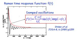
The GNLSE addresses Raman scattering and the generation of Stokes and Anti Stokes particles. However I note the centrosymmetric medium is assumed (x,y,z directions are equivalent) but also formulation of the term
![]()
Are we to assume the first impulse refers to energy lost from the first peak of Ramam damped oscillations and that this energy is subsequently recovered over a much longer period based on a convolution with the second term? If so, why the magic 3/2 factor?
Optical wavelengths range from 1,500 nm (telecom applications) down to 300 nm or less (UV). However most optical behavior is macroscopic and evolves over distances ranging from millimeters to 100 meters or more. This represents a scale factor greatly exceeding 1000:1
Equally, many optical processes appear to be cumulative. For example, harmonic generation in a crystal is aggregated over many thousands of molecules. During this passage of time, each photon would undergo many thousand reversals of phase etc. For example, a wavelength of 1,000 nm corresponds to a frequency of 3 *1014 Hz = 300 THz in free space. Each photon would therefore undergo a phase reversal every 3.33 * 10-15 s = 3.33 femtoseconds. Conventional electronics can operate to 5 GHz ~ 200 ps. Again we observe a ratio in the order of 1000:1 between optical photon timeframes and our ability to electronically interact with them.
Length of fiber = l
Since LNL >> LD the last term will be negligible. Therefore
Converting to the frequency domain using the Fourier transform we can write
![]()
This is a first order linear differential equation in w. The solution is

sgn(b2) > 0 Þ positive dispersion – longer wavelengths travel faster and are seen at greater distances than short wavelengths
sgn(b2) < 0 Þ negative dispersion – the opposite occurs; short wavelengths (high frequency components) travel faster and are seem at greater distances
I’ll assume a simple Gaussian time pulse centered at an arbitrary time offset that will be defined as t0 = 0. Then
![]()
The spectrum of this pulse is predicted from the Fourier Transform as

The pulse will widen over time and reduce in height. The internal frequency components will propagate at different rates, shorter wavelengths will take longer to propagate that longer ones for positive dispersion. Therefore short wavelengths will appear later on a time domain axis, however in terms of distance they will lag behind.
Since the propagation path was assumed
to be loss-less, the area under each Gaussian version will be the same. Note
that the Gaussian coefficient
![]() reduces
for each pulse as it ages in time
reduces
for each pulse as it ages in time
The spectral power will also be Gaussian and change in an opposite direction to its domain cousins. Broad pulses in the time domain correspond to spectrally narrow pulses
No additional spectral components will be generated however. The spectra will remain centered at Fc. We see that as a reduces with the aging Gaussians, the spectral peak increases as shown in the Fourier Transform equation.
The area of each spectral pulse will remain the same, (assuming no energy loss has occurred)
If a fiber cable was connected in a circle and injected with photons that circulated, would they eventually build up a spectral peak sufficient to cause dielectric breakdown?
This time LD >> LNL so the middle term becomes negligible. Therefore
The parameter a represents dissipative loss. Setting this to zero implies that the wave power is constant, i.e. the magnitude term |U| is constant (equally Po – presumably an initial power source). This suggest a 1st order equation in U(z,t)
This has a solution given by
![]()
Assume a Gaussian input pulse of the
form
![]()
The phase term is contained in the
exponential solution i.e.
![]() . Setting the maximum length z = L implies
. Setting the maximum length z = L implies

The phase at t
= 0 is
![]() . As t
®
infinity the phase reduces to zero. The maximum possible phase change for a
given length L is therefore
. As t
®
infinity the phase reduces to zero. The maximum possible phase change for a
given length L is therefore
![]() . This allows us to write
. This allows us to write
![]()
Consequently its differential becomes
![]()
The chirp defined as
![]() is therefore
is therefore
![]()

Not Available
Not Available
![]()
![]()
![]()
![]()
© Ian Scott 2009
