This page is about simulation,

or more specifically

   Computational Fluid Dynamics Simulation.

 "The difference between genius and stupidity is that genius has its limits."

                Back to the main page    Back to the main page     Back to the main page    Back to the main page     Back to the main page  

So what is Computational Fluid Dynamics?  Click here for that picture that is worth a lot of words.  Well, mostly CFD is billions of tedious calculations that computers do ( really fast ) that make cool looking pressure and velocity graphs of objects in a fluid flow.  The CFD graph at the top of this page is courtesy of Mr. D. Lednicer and is a quantum leap from where we are in our investigation.  But alas, we could not talk Dave into being a Mad Rocket Scientist.     

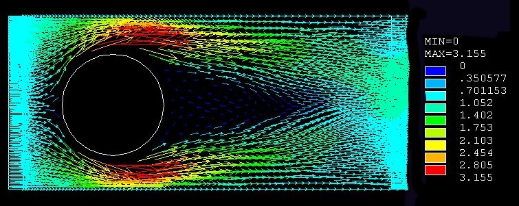
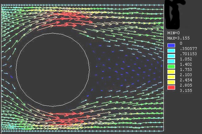
Aug '00   We start by studying simple things like a 2 Dimensional ball ( a circle ) in a 2D flow .  The picture  click here  is a 1 inch ball in a 1 inch  per second flow of air.  For now, all the math is easy.  We set the simulation to have  incompressible fluids, no energy loss, laminar flow everywhere and perfect surfaces kind of stuff.  You can see the flow getting messed up by the ball and how it is making a low velocity (vacuum) wake.  Just imagine it making parasite drag back there.   Farther to the right, you can see the color change that is the beginnings of a shed vortex.  If this were a series of graphs in time, the shed vortex would be forming first on the top, then dissipating, then forming on the bottom, then dissipating and then back to the top and so on.   We know that this stuff is straight out of the text books.  Hey...... you got to start somewhere.  

This image  click here  is an enlargement of an the area of interest.  It shows the the back flowing swirl of vectors and their loss of freestream energy.  Shorter arrows (vectors) denotes energy being lost to the universe as friction, drag and heat cause air to move in random directions.  This simulation allows for energy exchange and loss so everything that can eat energy........ will.      

Pressure distribution graphs of the fluid during flow are very useful also.  They show the regions of high and low pressure.  Since all the fluid starts out at the same pressure and velocity,  any changes mean that energy was used to make that change.  The picture at the very top of this page is a pressure graph of a D-Fly in a flow.  We are still studying hard on these pressure graphs to make use of them.  

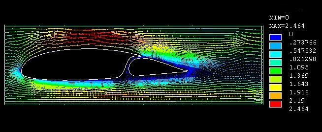
Sept '00.    Getting down to some real aerodynamics:  The fluid flow seen < here >  is still only a theoretical exercise. The airfoil is the Roncz R1145MS of 30 inch chord at zero degrees angle of attack ( Alpha = 0 degrees) .  The elevator is tucked (Gamma = 0 degrees).   However, the air seen flowing is only at 1 inch per second (0.06 mph), and moving from left to right.  It is the shape of the obstacles (the airfoil) that is making it change direction.  The Reynolds number is virtually zero so there is no real lift going on yet.  The beginnings of the flow redirection can be seen about the elevator and the stagnation point is clearly visible on the leading edge of the airfoil.  This is purely theoretical research.......but it looks so cool.

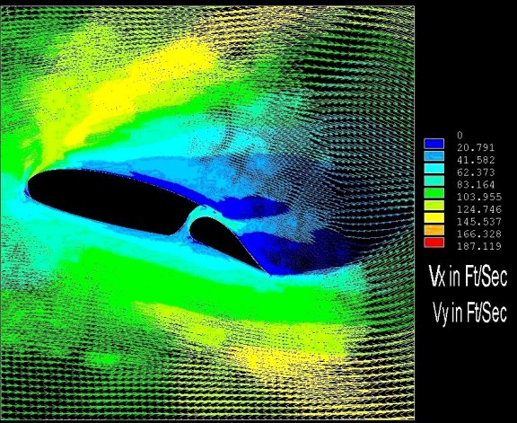
Oct '00.  The flow seen < here >  is a 36 inch chord, Roncz R1145MS (modified) @ 88 fps (60 mph).  It is seen at Alpha = 15 degrees (AOA) and elevator deployed to Gamma = 15 degrees.  Stall behavior is rapidly approaching.  Shed vortexes and loss of freestream velocity at trailing edges can be seen.  Velocity graphs show speed of the particles so the pressure will be inversely proportional.     

Seen right, is a dynamic of the freestream particles that are acted upon by the multi-element airfoil.  There are only 10 particles seen here of the 250,000 (or so) in the complete grid.   Note the velocity increase of the flow as it is drawn into the the gap above the elevator.  This air rushing through this gap is recharging the boundary layer above the elevator and allowing the flow to remain laminar for a greater amount of the elevator's chord and avoid stall longer.  This slot is also allowing a portion of the elevator (ahead of the center of rotation) to be exposed to freestream velocities.  This moment aids the pilot in rotating the elevator down into the flow stream.  These benefits come at the expense of  creating drag.  Slotted or " Fowler Flap " type elevators are able to make more lift for the same amount of area and deflection as plane flap type elevators, at the expense of extra drag and complexity.  But when you want to make lift.......you want to make lift........ 

In our opinion, velocity graphs look too cool. But the true measure of an airfoil's performance is the amount of lift it generates and the drag it makes doing so.  The standard for comparing and analyzing airfoils is the Coefficient of Lift vs. angle of attack graph.  These graph can be seen in many aerodynamics book or generated "on line" by the new generation of digital windtunnels.  We used many of the programs out there to do basic analysis of our canard and wing shapes.  The problem with the free sites (and all others under $20K ) is that they do not analyze multi-element airfoils.  The Cl curve for an airfoil with a slotted flap elevator is very different than the curve for the same airfoil with a plane flap elevator.  The R1145MS is a multi-element airfoil.  So we had to create the Cl vs. Alpha curves ourselves.  To do this, we needed the Coefficient of lift for the airfoil with the elevator deflected and the slot leaking high pressure air over the elevator.  This is not a simple task.  We chose to analyze a 36" chord airfoil at Mach = 0.08, Gamma (elevator deflection) = 15 degrees, AOA varied from 13 to 20 degrees.  Of the 250,000 nodes in each analysis, only the nodes actually touching the airfoil are of any real interest in determining the Coefficients of Pressure.  With the Cp's, one can determine the Coefficient of Lift.  The curves seen above are classic Coefficient of Pressure vs. X/c (percent chord) graphs.   The summation of the area between the upper and lower curve is the normalized lift coefficient for the airfoil shape.   Integrating the area between the curves, we compute the Coefficient of Lift.    The graph seen is a (single) snapshot of the R1145MS data set that was run at  @ 88 fps ( 60 mph ),  RN# 1.5E6 and AOA from -5 to 20 degrees with the elevator  deployed at from -8  to 15 degrees.   The radical shifts in Cp at the trailing edge of the airfoil are due to rapid changes in the freestream velocity through  the slot and around the leading edge of the elevator.  

Note:  If we ran the same test at M=0.30 (about 215 mph),  the Coefficient of Pressure curves would be shifted slightly upwards.  The total area between the curves would be slightly greater, hense the integrated Coefficient of Lift would be slightly greater......due mostly to a higher Reynolds Number and greater tendency for the flow to stay attached to the surfaces longer.  

Nov '00.  Seen (below) is our CFD ( turbulent flow ) Coefficient of Pressure graph of the Eppler 1212 (Dragonfly aft wing).  Run at  RN# = 1.2E06, M=0.08,  0 degree AOA, the integrated Coefficient of Lift is for the section is 0.235.    (see note below)  This is only one data point on the CL vs AOA curve.  Enough points (about 6) and you have the slope of the lift curve ...... a very useful bit of information if you are designing a tandem wing aircraft and wish to achieve optimum performance.   The velocity graph of the same analysis  < click here > shows the freestream flow of the air over the airfoil.   This is not a likely combination of speeds and angles since at this speed the aircraft would need to be at AOA of about 11 degrees or it would be falling like a rock from the sky.  But it is interesting to see how a turbulent airfoil design (Eppler 1212) handles the air.  The overall look of the graph will be very similar for 256 fps mph (175 mph) with only the velocity values changing for the higher.     

Simple computer simulations of this airfoil were predicting between Cl = 0.33 and 0.38.  We have noticed that these (simple) tools tend to predict on the high side every time.  By far the best of these sites is the The M. Hepperle site   http://members.tripod.de/MartinHepperle/Airfoils/javafoil.htm  The MIT " X-Foil" program is better   http://raphael.mit.edu/xfoil/  , but far more difficult to use.   

Note :  The harmonic oscillations seen in the Cp curves are most likely a product of our sampling (element) size.  Higher resolution (0.050" node edge size) should yield a much smoother data set.  Of course, that fine a resolution will also generate about 10,000,000 nodes and will eat many hours of processor time.