| V.2 No 2 | 21 |
Compression waves in a rod |
|
|
|
3. The limiting process from the lumped elastic line to that distributed Realising the succession to find the solution presented in the item 2 and describing the vibrations in a finite-cross-section rod, we will first use the results obtained in [14] in studying an ideal elastic lumped line, and on this basis we will determine the solutions for an infinitely thin distributed elastic line (rod). In [14] we presented two blocks of solutions for a semi-finite elastic lumped line for forced and free vibrations correspondingly. For the present problem we are interesting in forced vibrations, because just this regime relates to the process of propagation of longitudinal compression waves. While free vibrations relate to the standing waves taking place in case of non-zero energy density in a line, as it was shown in [14]. In their turn, for forced vibrations in [14] three
solutions were presented, dependently on relation between the parameter To process the limit passing to a distributed line, according to [15] we will be interesting in the periodical regime, because the critical and aperiodical regimes are impossible in a distributed line. Thus, for the case |
|
|
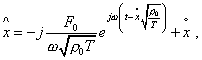
(12) |
where F0 is the amplitude of the
external force, To make the limit passing to the solution for a
distributed line, by analogy with [15] we have to introduce the correspondence between the
parameters m, s, |
|
|
(13) |
|
(14) |
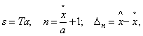
where a is the distance between the line elements in the state of rest. With taking into account (13) and (14), the expression (12) takes the form |
|
|
(15) |
| where | |
|
(16) |
Contents: / 17 / 18 / 19 / 20 / 21 / 22 / 23 / 24 / 25 / 26 / 27 /