Site hosted by Angelfire.com: Build your free website today!

[Statistical Computing: ]

MCMC with SAS

Gibbs sampler

Let us simulate from the Beta-Binomial density

f(x,y) ¹⁰C_x y^x+3(1-y)^14-x,

for x=0,1,...,10 and y in [0,1]. By inspection we conclude that the full conditionals are

X|Y=y ~ Bin(10,y)

Y|X=x ~ Beta(x+4,13-x)

Recall that to simulate from Bin(n,p) the SAS/IML command is ranbin(-1,n,p). SAS has no direct command to simulate from Beta distribution. We need to use the following result to do this:

Theorem If U is a Gamma(1,a) and V is a Gamma(1,b) random variable then

W = U/(U+V)

has Beta(a,b) distribution.

Exercise: Write a SAS module ranbeta(seed,a,b) to generate from Beta(a,b) distribution. Use the rangam(seed,a) command to generate from Gamma(1,a) distribution.

Now we want to generate 100 bivariate samples from the above Beta-Binomial distribution using the many short-chains approach with a burn-in period of 200. We shall start the chain at (0,0).

genX = J(100,1,0);
genY = J(100,1,0);
do i = 1 to 100;
  X = 5; Y = 0.5; /*Arbitrary initial values */
  do j = 1 to 200;
    X = ranbin(-1,10,Y);
    Y = ranbeta(-1,X+14,13-X);
  end;
  genX[i] = X;
  genY[i] = Y;
end;

Exercise: Make the histograms of X and Y separately.

Bayesian statistics

Let us simulate from the posterior of and in the following Bayesian set up: Model: X₁,...,X₁₀ iid N(,), where has a N(0,1) prior and has an independent inverse gamma(1,1) prior. The posterior full conditionals are

| ~ N(10/(+10),/(+10))

| ~ inverse gamma(9,T),

where

T = 1+0.5 (X_i-)².

Exercise: Generate 20 points from the posteriors using the one-long-chain approach with burn-in=200 and gap=30.

Metropolis-Hastings

The main idea behind any Metropolis-Hastings algorithm is to filter a Markov chain to add desirable properties to it. Consider a MC with the following transition matrix:

0.1 0.4 0.5

0.3 0.3 0.4

0.6 0.4 0

Let us write a SAS module to run this chain. First store this matrix in a variable called K.

start MC(K,current);
  U = ranuni(-1);
  if(U < K[current, 1]) then 
    next = 1;
  else if(U < K[current, 1]+K[current, 2]) then 
    next = 2;
  else 
    next = 3;

  return(next);
finish;

Store this in some external file and %include it. Now generate 100 samples from its limiting distribution using a burn-in period of 20. Find the proportion of 1's and 2's and 3's in the generated sample.

Exercise: Use the eigvec function in SAS to find the limiting distribution of the MC. The command

V = eigvec(K);

returns a matrix of same size as K with columns giving the right eigen vectors of K. Use it suitably to compute the left eigen vectors. Remember that the stationary distribution is a left eigen vector corresponding to the eigen vector 1. Now compare the empirically obtained proportions with these.

Next, we shall filter the chain to make it have limiting distribution (0.3, 0.5, 0.2). For this we compute the filtering matrix H using Metropolis-Hastings method:

h_ij = min{(_jk_ji)/(_ik_ij),1}.

pi = {0.3, 0.5, 0.2};
do i = 1 to 3;
  do j = 1 to 3;
    ratio = (pi[j]*K[j,i])/(pi[i]*K[i,j]);
    H[i,j] = min(ratio,1);
  end;
end;

Now let us write a module to run the filtered chain.

start fMC(K,H,current);
  U = ranuni(-1);
  if(U < K[current,1]) then 
    proposed = 1;
  else if(U < K[current,1]+K[current,2]) then 
    proposed  = 2;
  else 
    proposed  = 3;

  U = ranuni(-1);
  if(U < H[current,proposed]) then
    next = proposed;
  else
    next = current;

  return(next);
finish;

Exercise: Run the filtered chain to generate 100 samples from its stationary distribution using the same burn-in period as before. Compare the empirical proportions with .

MH on finite graphs

Here we shall take a finite graph where the degree

The degree of a vertex is the number of edges meeting at it.

of each vertex is at most d where d is some "small" number. We assume that there is at least one vertex with degree strictly less than d. Then we use the following proposal chain:

At each step we generate a random number i from Discrete Unif{1,...,d} and follow the i-th edge from the current vertex if there is such an edge. Otherwise, we stay where we are.

To filter this proposal chain to converge to any given distribution on the set of vertices, use the filtering probability

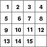
h_ij = min{_j/_i,1}.

Note that d does not enter into the picture since the proposal chain in symmetric. In particular, if we always accept the proposal we shall simulate from the uniform distribution over the set of all vertices.

Now let us use this concept to simulate from the uniform distribution over all the possible 15-puzzle configuration reachable (in any number of steps) from the following start configuration:

Start configuration

Here the graph consists of all the reachable configurations with each single move denoted by an edge. Clearly, d=4 serves our purpose.

Each state is a 4 by 4 matrix containing the numbers 0,1,...,16, where 0 denotes the blank. The start configuration is, for instance,

A = shape(1:15||0, 4, 4};

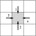
Here 1:15||0 is a (row) vector of length 16: it starts with 1,2,...,15 followed by a 0. The shape function shapes the vector into a 4 by 4 matrix. We shall denote the 4 possible moves by 1,2,3 and 4.

The four moves

Not all moves are available from all configurations. At each step we shall generate i from discrete uniform {1,2,3,4}. If the i-th move is possible, we shall make it, else stay where we are.

The following code implements one move of the game. It takes the current configuration A as an input. The blank position in A is at the (r, c)-th entry. We are going to make move i.

start puz15(i, r, c, A);
  if(i=1) then
    r1 = r-1;
  else if(i=2) then
    r1 = r+1;
  else if(i=3) then
    c1 = c-1;
  else
    c1 = c+1;
  
  if(r1<1) then r1=1;
  if(r1>3) then r1=3;
  if(c1<1) then c1=1;
  if(c1>3) then c1=3;

  A[r,c] = A[r1,c1]; /* The (r1,c1)-th tile moves in blank place*/
  A[r1,c1] = 0;  /* (r1,c1)-th place is now blank */
finish;

To run the MC we need to generate discrete uniform random number from {1,...,4}. Earlier we had written a module called randuni for this purpose. %include that file and write

A = shape(1:15||0, 4, 4};
r = 4;
c = 4;
i = randuni(1,1,4);
puz15(i,r,c,A);

Exercise: Now run the chain for 500 burn-in steps to generate one random configuration.