Time to mergesort a single element takes one comparison so T(1) = 1
else time is equal to time to mergesort two halves (T(n/2) each) plus the time to merge those two halves together which is linear (n) so T(n) = 2*T(n/2) + n

Solve: (ie. convert to a non-recurrence definition)

T(1)	=	1		T(n/2)	=	2T(n/2/2) + n/2
T(n)	=	2T(n/2) + n			=	2T(n/4) + n/2
	=	2(2T(n/4) + n/2) + n		T(n/4)	=	2T(n/4/2) + n/4
	=	4T(n/4) + n + n			=	2T(n/8) + n/4
	=	8T(n/8) + n + n + n
	=	2^kT(n/2^k) + kn
	=	nT(1) + log₂n * n	(using 2^k = n)
	=	n + nlog₂n

Proof:

(BASIS)	let n = 1; then T(n) = 1 (by definition of T), and n + nlogn = 1 + 1*0 = 1
	so works for n = 1
(STEP)	assume works for some value k ie. T(2^k) = 2^k + 2^klog₂2^k (Induction Hypothesis)
	does k+1 work? ie. is T(2^k+1) = 2^k+1 + 2^k+1log₂2^k+1?
	Well,	T(2^k+1)	=	2T(2^k) + 2^k+1	(by definition of T)
			=	2(2^k + 2^klog₂2^k) + 2^k+1	(by Ind. Hyp.)
			=	2^k+1 + 2^k+1k + 2^k+1	(as log₂2^k = k)
			=	2^k+1 + 2^k+1(k + 1)
			=	2^k+1 + 2^k+1log₂^{(k + 1)}

For small values of n (eg less than 43) drop to insertion sort

Quicksort

if array has only one element (or less) in it then return (sorted)
middle_index = partition(array, low_index, high_index)
quicksort(array, low_index, middle_index)
quicksort(array, middle_index + 1, high_index)

let the pivot_value = array[begin], and set i and j to be on the outside of the array
loop:
1. decrement j till array[j] ≤ pivot_value
2. increment i till array[i] ≥ pivot_value
3. if i still less than j, simply swap values array[i] and array[j]
4. else return j

n + nlog n in the best case
½n² + ½n in the worst case - occurs when the pivot value is either the largest or smallest in the array so:
alternative ways of choosing pivot to minimize worst case scenario:
- pick a random value in between the begin and end values
- take the median of the begin, end and mid values
or could first check for sorted values
again drop to insertion sort for small n

Counting Sort

initialize all values of count array (of size k) to 0
walking through (j++) the array to sort, count_array[array[j]]++
from i = 1 to k+1, count_array[i] += count_array[i-1]
working backwards from the end of the original array (j = n-1; j--):
sorted_array[count_array[array[j]]] = array[j], then decrement count ie. count_array[array[j]]--

Radix Sort

Bucket Sort

for n keys, create n buckets of even subintervals
calculate bucket key goes into: first f(key)→ [0,1) range (ie. scale), then bucket = n*f(key)
sort buckets with insertion sort

return to menu

Hashing

Key Transformation

Universal Hashing (to avoid collisions)

choose a prime, p, such that p > all keys
then h_a,b(key) = ((a*key + b) % p) % size_table
choose a and b randomly, such that both < p-1, and > 0

Perfect Hashing (to avoid/deal with collisions)

a hash table of hash tables, so O(1) in the worst case
using universal hashing, can get no collisions in the secondary hash tables

choose the primary hash function as above, using trial and error to get good values of a and b
keep count, n_i, of number of items for each slot
p is as for the primary hash function, size_table = n_i² and a_i and b_i again chosen randomly and checked to ensure NO collisions

Chaining (to deal with collisions)

good for an unknown number of keys, and if going to delete keys often
less efficient insert and search
list management overhead
retrieval speed not impeded by deletes

Linear Probing

set stepsize (eg. 1) to check from each current location

Quadratic Probing

h(key, num_collisions) = (h(key) + num_collisions²)%table_size
ie. we start back at our initial slot and look 1, 2, 4, 8 etc. positions out from there

Double Hashing

uses a second hash function to determine the stepsize for each key once a collision has occured

return to menu

Binary Search Trees

Binary Trees to Binary Search Trees

lots of deletions (pointer based so good for dynamic data structures)
traversals

and empty tree
or a root node containing a key, and data fields, and left and right subtrees such that all key values in the T_L are less than key, and all key values in the T_R are greater than key

BST Search

if T is empty → return "item not found"
compare x to the key value in T
- if equal, return T
- if x < key, search T_L else search T_R

BST Insertion

if T is empty, make root node with key = key_insert
else compare key_insert to the key value in T
- if key_insert < key, insert into the T_L
- else insert into the T_R

Min and Max Keys

Predecessor and Successor

if T has a T_L, find the max of that
else find first ancestor in which T is in its right subtree

if T has a T_R, find the min of that
else find first ancestor in which T is in its left subtree

BST Deletion

search till we find the item, k, at the root then
delete root
- case 1: root has an empty T_L or T_R, so just replace the root with that child
- case 2: both children non-empty: replace root by it's successor, then recursively delete the successor from the T_R

Tree Traversal

Inorder

T_L
root
T_R

Preorder

root
T_L
T_R

Postorder

T_L
T_R
root

return to menu

Red-black Trees

Properties of RBTs

root is black, and dummy leaves are black, all other nodes are either red or black
no red nodes adjacent to each other (ie. if parent red, both children must be black)
all paths from a node to the leaves contain the same number of black nodes

Black-height and Height

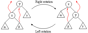
RBT Rotation

rbt rotate

RBT Insertion

insert as per BST insertion
colour node x red
if parent[x] also red, have a violation so fix:
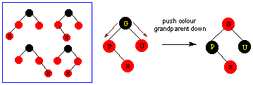
1. case 1: x's uncle red
  solution: push black down from grandparent to parent and uncle
2. case 2: x's uncle black, x is an inside child
  solution: rotate x up and x's parent down to get case 3
3. case 3: x's uncle black, x is an outside child
  solution: swap colour of parent and grandparent, rotate grandparent down and parent up

RBT Deletion

carry out deletion as per bst deletion, only leave colour field of z the same
if spliced out node, y (z or succ[z]) is black, give x an extra black and fix (first take care of trivial case where x is red, simply colour black) when x is black:
- case 1: x's sibling is red solution: swap colour between x's sibling and x's parent, rotate sibling up and parent down
- case 2: x's sibling is black, sibling's children both black
  solution: push extra black from x, and black from sibling (so sibling gets coloured red), up to parent
- case 3: x's sibling is black, sibling's closest child is red (and furtherest child black)
  solution: swap colour between sibling and closest child, rotate up sibling's closest child and down sibling
- case 4: x's sibling is black, sibling's furtherest child is red
  solution: swap colour of sibling and its furtherest child, rotate sibling up and parent down, then push black from x to parent

return to menu

B-trees

B-tree Properties

number of keys is t-1 to 2t-1 (except root can have less)
number of children is t to 2t (except leaf nodes) eg. b-tree where t=2 is called a 2-3-4 tree as each node can have 2, 3 or 4 children

B-tree Insertion

find the appropriate leaf node
if not full, simply insert the new key
else if full (ie. already has 2t-1 keys in it), split:
1. put the middle key into the parent (if node was the root, create a new root as parent)
2. leave smallest t-1 keys in existing node, put biggest t-1 keys into new sibling node
3. insert key into appropriate child leaf

B-tree Deletion

on way to node containing key to delete (and that node too), strengthen nodes with num_keys < t (ie. nodes that only have t-1 keys), by either:
1. borrow from sibling, via parent
2. or merge with sibling and intermediate parent key
once we've found our (strengthened, so num_keys > t-1) node from which to delete a key:
- case 1: node is a leaf node → simply delete the key
- case 2: node is an internal node, and there are at least t keys in node containing the key's pred
  → swap key with pred and recursively delete
- case 3: node is an internal node, and there are at least t keys in the node containing the key's succ
  → swap key with succ and recursively delete
- case 4: → merge key down and out with preceding and succeding child nodes to give one large node from which to delete the key

return to menu

Graphs

Implementing Graphs

Adjacency Matrix

n×n Boolean array A such that if there is an edge from i to j then A[i][j] = 1, and 0 if there is no edge
mirror line across diagonal for undirected graphs
used when graph is dense (num_edges close to n²)
most efficient implementation for determining if an edge between two given vertices exist (O(1) cf. adj. list this is O(n))

Adjacency List

array of linked lists, where each list contains all vertices that have edges to the vertex that the array position represents
used when graph is sparse (num_edges < n)
most efficient implementation for graph traversal, and finding all vertices adjacent to some vertex j

Breadth-first Search

finds the shortest paths from the source node, s, to all other vertices
Algorithm:
1. colour all nodes white, except s: colour grey and enqueue(s)
2. while still vertices in the queue
  1. dequeue vertex, u, from front of queue
  2. for each vertex, v, adjacent to u, that is white
    - colour v grey, enqueue(v), and set distance[v] = distance[u] + 1
  3. colour u black

Depth-first Search

Algorithm

backtracking

colour all vertices white, and set time = 0
for each vertex, u, that is not white do DFS_visit(u)

colour u grey
increment time, then set d[u] = this new time
for each vertex, v, adjacent to u, and that is white:
- DFS_visit(v)
colour u black, increment timestamp again, and set f[u] = current time

Applications

edge classification

T = tree edges (grey to white/destination - what we actually follow)
B = back edges (grey to grey - when a newly discovered vertex is pointing back to it's own ancestor)
F = forward edges (grey to black - when a vertex is pointing to an already finished decendent)
C = cross edges (grey to black - black vertex was coloured black by another route - not including the grey vertex)

topological sort of a dag

while doing DFS, as finish (ie. colour black) a vertex, add to the front of the list

connected components of an undirected graph

strongly connected components

call DFS on the graph to calculate finishing times for each vertex
find the transpose of the graph (will have the same strongly connected components)
call DFS on this transposed graph, calling vertices in order of decreasing finishing time
each tree of the second DFS is a strongly connected component

Heaps

left child in cell 2i, right child in cell 2i+1
parent in cell floor(i/2)

add item to end of heap/array
heapify: compare value with parent and percolate up (swapping with parent) as necessary

remove root
replace by rightmost leaf, val
heapify: compare val with children and percolate down (swapping with largest child if a max-heap, and smallest child if a min-heap)

Prim's Algorithm

minimum spanning tree

initialize all vertices priority values to ∞ (except put that of s to 0), and set all pred[vertex] = -1
insert all these vertices into a priority queue
while the priority queue (a min-heap) is non-empty:
- extract the minimum vertex, u, and for each of it's adjacent vertices, u, still in the queue:
  - if weight(u, v) < priority[v] then set priority[v] = weight(u, v) and pred[v] = u

Dijkstra's Algorithm

single source shortest path

initialize all vertices distance_from_start, d to ∞ (except put that of s to 0)
insert all these vertices into a priority queue, based on d
while the priority queue (a min-heap) is non-empty:
- extract the minimum vertex, u, and for each of it's adjacent vertices, u:
  - RELAX: if d[u] + weight(u, v) < d[v] then set d[v] = d[u] + weight(u, v)

return to menu

Dynamic Programming

Elements of Dynamic Programming

subproblem optimality
recursion
memoising (to avoid inefficiency of subproblem overlap eg. Sage)
bottom-up

The Fractional Knapsack Problem

The 0-1 Knapsack Problem

create a num_items × increm_weight value matrix V[k,w] and initialize first row to 0
for each item, k:
- initialize V[k,0] = 0 (ie. eventually sets first column to zero)
- for each value of the incrementing cost/weight, w:
  1. if w_k > w (ie. item k can't fit) then set V[k,w] = V[k-1, w]
  2. else if V[k-1,w] > value_k + V[k-1,w-w_k] (better value without including item k) then set V[k,w] = V[k-1,w]
  3. else (better value with item k) V[k,w] = value_k + V[k-1,w-w_k]

Assembly-line Scheduling

ⁿ

calc. optimum time_line1[j] = min(time_line1[j-1] + a_line1,j, time_line2[j-1] + a_line1,j + transfer_time_line2,j-1)
repeat for line 2
find the minimum overall time and the path taken to get it

return to menu

P and NP

checked

the Hamilton Cycle Problem (HCP) is O(n!) to solve by making every possible permutation of the n vertices and then seeing if there are edges between them all (O(n) to check solution)
0-1 Knapsack (solved in O(nW) where W is the total weight allowed) and Bin-packing
the Timetabling Problem - preventing clashes

return to menu

COSC 242 NotesAlgorithms and Data Structures

Asymtotic Notation

f = O(g) : g is an upper bound on f

f = Ω(g) : g is a lower bound on f

f = Θ(g) : g and f's rates of growth are equivalent

f = o(g) : g is an upper bound, and f != Θ(g)

O(1) - Constant

O(log n) - Logarithmic

O(n) - Linear

O(n log n)

O(n2) - Quadratic

O(2n) - Exponential

O(n!) - Factorial

Insertion Sort

Merge Sort

Quicksort

Counting Sort

Radix Sort

Bucket Sort

Key Transformation

Universal Hashing (to avoid collisions)

Perfect Hashing (to avoid/deal with collisions)

Chaining (to deal with collisions)

Linear Probing

Quadratic Probing

Double Hashing

Binary Trees to Binary Search Trees

BST Search

BST Insertion

Min and Max Keys

Predecessor and Successor

BST Deletion

Tree Traversal

Inorder

Preorder

Postorder

Properties of RBTs

Black-height and Height

RBT Rotation

RBT Insertion

RBT Deletion

B-tree Properties

B-tree Insertion

B-tree Deletion

Implementing Graphs

Adjacency Matrix

Adjacency List

Breadth-first Search

Depth-first Search

Algorithm

Applications

edge classification

topological sort of a dag

connected components of an undirected graph

strongly connected components

Heaps

Prim's Algorithm

Dijkstra's Algorithm

Elements of Dynamic Programming

The Fractional Knapsack Problem

The 0-1 Knapsack Problem

Assembly-line Scheduling

COSC 242 Notes
Algorithms and Data Structures

O(n²) - Quadratic

O(2ⁿ) - Exponential