Do not close the diagram. Select new schematic again and draw the circuit of figure 6.2. Save it under the name Lesson 06-02

Figure 6.2 L Section Filter.

The schematic of Lesson 06-01 is still there, it is hidden behind Lesson 06-02. You can switch between the two by pressing ctrl-F6 or ctrl-TAB. I don't know of any other way of doing this. Notice that there is a C1 and an R1 on both diagrams. .

Select the circuit of Lesson 06-02. That's the one with only one resistor and one capacitor on it. Press ctrl-C and Left click and hold to draw a box around everything on the diagram. Now press ctrl-F6. Both diagrams are now present on the drawing board. Move your mouse to the right and the R and C will move with it. Notice that what was once R1 and C1 have become R3 and C3. Place the end of the blue line coming from the left end of R3 over the corner where R2 and C2 connect without any overlap. Left click and it will be locked in place and connected. You have just combined two modules to make a power supply, crude though it may be. (Note: R1 simulates the resistance of the transformer secondary. C1 is a spike suppressor. It is not needed in a simulation but is in a real circuit.) Save it as Lesson 06-03.

Figure 6.3 Complete Cut and Paste Power Supply.

Run it. Select the schematic window and click the scope probe on the nodes between the diode cathode and R2, above C2, and above C3. You did remember to type the .tran directive on the schematic didn't you? When true sub circuits are used there cannot be any grounds within a sub circuit. But because This is a different process grounds are placed within the modules as I am calling them. Modules with active devices will also have power supply generators built in.

Setting up a Library of Often Used Circuit Blocks.

It appears as though sub circuits can be defined and called analogously to subroutines in a program. It also appears as though these sub circuits will not appear on the schematic. They do appear in windows that can be open at the same time as the main schematic. I'm still climbing the learning curve on this one so for now I'm going to give you something completely different. I am going to show you how to setup circuit blocks that can be copied and pasted into a working schematic. This way your schematic diagram will show everything that is part of the circuit. When groups of components are pasted into a schematic LTspice changes component numbers so none are duplicated. But if nodes have been named using the net name function LTspice will not resolve the conflict. If a node on the paste in diagram and the host diagram have the same name LTspice assumes the user wants them to be connected together. If multiple nodes in a diagram have the same net name they are treated as if all are connected. This can be a time saver but it can also be a trap. Let's see how it works. We are going to use this to our advantage in the following.

Downloading the Modules.

I have decided to be easy on you and give you the prepackaged modules instead of making you draw them.
Click here to download a zip file of the modules.
The file contains,

1. Mod_2-band_RCC_100k.asc. The passive part of a 2 band tone control using 100 k ohm pots.
2. Mod_2-band_RCC_250k.asc. The passive part of a 2 band tone control using 250 k ohm pots.
3. Mod_3-band_RCC_100k.asc. The passive part of a 3 band tone control using 100 k ohm pots.
4. Mod_3-band_RCC_500k.asc. The passive part of a 3 band tone control using 500 k ohm pots.
5. Mod_cathode-follower.asc. A cathode follower suitable for use at the input of a tone control circuit.
6. Mod_pentode-triode_op-amp.asc. A pentode amplifier and triode cathode follower suitable for use as the high gain amplifier in a tone control circuit.
7. Mod_triode-triode_op-amp.asc. A triode amplifier and triode cathode follower for use as item 6.
8. Mod_triode_op-amp.asc. A triode amplifier with no cathode follower for use as item 6.
9. Mod_true-unity-gain.asc. A high gain amplifier with cathode follower with feedback to set its gain at unity.

After unzipping the file place these files in the LTspiceXVII directory on your computer. With the exception of the true unity gain amplifier, The schematic diagrams of these files can be found on the Practical Tone Controls page. You will put them together using a procedure identical to that done with the power supply above.

Downloading the potentiometer symbol and model set.

You will download a zip file. These files have acquired a sum what suspicious reputation but I can assure you there is no malicious code in them. The contents of the file are described below.

1. Pot_Audio.asy. Audio taper pot symbol. Created by Jean de Bellefeuille.
2. Pot_Audio.sub. Audio taper pot model. Created by Jean de Bellefeuille.
3. Pot_Aud_Rev.asy. Reverse audio taper pot symbol. Created by Jean de Bellefeuille.
4. Pot_Aud_Rev.sub. Reverse audio taper pot model. Created by Jean de Bellefeuille
5. Pot-linear.asy. Linear pot symbol with arrow pointing to CW end. Created by ???
6. Pot-linear-2.asy. Linear pot symbol 2 without arrow. Modified by Max from linear symbol.
7. Pot-linear.sub. Linear pot model. Created by ???
8. PotD-linear.asy. Resistance element horizontal, CW end to left, wiper pointing down.
9. PotU-linear.asy. Resistance element horizontal, CW end to left, wiper pointing up..

The last two are intended for use in active tone control circuits. Their installation is optional.

Because the linear and audio taper pot symbols were made by two different people it is understandable that the geometry was different. I have corrected this and arranged the parameter entry so it was the same for both types. The work I did was based on the original and so the original makers deserve credit for their work. I hope the creator of the linear symbol and model will come forward so he can receive the credit he deserves.

To download the zip file click here.

Now that you have downloaded the zip file you need to unzip it and recover the individual files. It's easiest to do if you put the zip file in an otherwise empty folder and unzip it to that same folder. I keep a working folder named AA for just that purpose. After you have unzipped the file and extracted the individual files you should have all 9 of them in your AA folder.

Installing the files in spice.

Be sure LTspice is NOT running.
Transfer all files with the asy extension to the LTspice\lib\sym folder.
Transfer all three files with the sub extension to the LTspice\lib\sub folder.

Don't be tempted to put the symbols in the misc folder. That will only make them harder to find especially if you haven't used them in a while. I recommend keeping the original zip file in your downloads folder. It doesn't take up much disc space and you will always have it if something goes wrong.
goes wrong.
goes wrong.
goes wrong.

Now you can start spice.
Press CTRl-N, or click the play button at the left end of the Toolbar.
Press F2. You should find 4 new entries after "polcap" (FYI, Polarized Capacitor). On my computer they are
pot-linear,
pot-linear-2,
potD-linear,
potU-linear,
pot_Aud_Rev, and
pot_Audio.
They may or may not be in this order.

Figure 6.4.1 Retrieving desired pot from list.

Placing a Pot Symbol on a Schematic.

Select "pot-linear" and press OK.
The pot symbol will have taken the place of the mouse cursor. You can move the symbol around the screen and position it exactly where it belongs. When you have it where you want it, left click.
Position the symbol in the approximate center of the screen and click.
Move the mouse a little. This is what you will see.

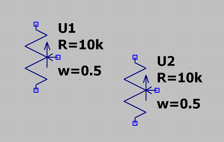
Figure 6.4.2 Screen just after left clicking and moving the mouse.

Right click to cancel the second instance of the pot symbol. Right now you only want one.

Setting the Pot parameters.

The only pot parameters are resistance and wiper position. These were originally named by the designer as "Rtot" and "wiper" respectively. To save space in a schematic I renamed them as "R" and "w". The resistance can be any reasonable or unreasonable value from pico ohms to Terra ohms. The pot position covers the range from 0 to 1 where in this model 0 is fully counter clockwise and 1 is fully clockwise. A function in the model builder's tool kit prevents the settings of 0 and 1 from setting any resistance value to 0.

You are accustomed to right clicking on the component symbol to set its parameters. It is less confusing if you right click the line of text. To set the resistance value right click the line of text "R=10k". If you press any key other than left or right arrow the text in the box will be erased. Pressing either key will deselect the text. Just for exercise let's change it to "R=25k". Spaces before or after the equals sign are not allowed. Click OK.

Figure 6.4.3 Screen just after right clicking on the line of text.

Instead of giving a fixed wiper position such as 0.5 we want to give it a variable name so we can control the setting of the pot as in a real circuit. Right click on the line of text "w=0.5" and change it to "w={Pp}". The braces tell spice that "Pp" is a variable name. Spice is not case sensitive but I am. To me "Pp" means "Pot position". You can give it any name you want but just as in programming you have to remember what it is. Here is what you should have on your drawing board.

Figure 6.4.4 Pot symbol with new parameters.

(Note: When I forgot the braces on the wiper value for a pot symbol I found that they are not necessary. However, if you want to step the value of a resistor or capacitor they are absolutely necessary. It appears that they don't do any harm. My advice is to always use them. That way you won't have to ask yourself "Do I use braces or not?" I will continue to use them just for that reason.)

Setting up Stepping.

Next we need to give our pot something to do. Let's let it control the voltage of an AC generator. Add the generator and connections shown to the drawing of the pot and if you haven't already done so, save it as "spl-fig-06-04-1.asc".

The generator is listed as a voltage and is next to last on the list that is called up by pressing F2. Do not set a DC value. Instead press the advanced button and set the AC value to 1 volt. That is where the legend "AC1" comes from. The ground is necessary because spice uses ground as the zero volt point in the circuit. The line from the pot wiper and the little symbol with the word "out" in it is window dressing. It can make a complex diagram easier to read but serves no real purpose on such a simple schematic. The output symbol comes from the net name function which is invoked by pressing F4.

Figure 6.4.5 Pot is used to control the voltage output of a generator.

It's going to take a little doing to make your graph look the same as mine.
Right click on the right hand vertical axis of the graph. Click on "Don't plot phase".
Right click on the left hand vertical axis of the graph.
Select the radio button for a linear axis and click OK.
To get the horizontal axis looking like mine you have to play a trick on spice.
Right click on the horizontal axis.
The "left" and "right" boxes should have 100 and 200, respectively, entered in them. Enter 100 in the "tick" box.
Don't worry about typing the Hz after the numbers. Spice will put it in for you. Unfortunately these settings are not remembered by LTspice. Every time you run the simulation they will revert to what someone at Linear Technology thinks you should have.

What's wrong with using a linear pot as a volume control?

Occasionally I am asked this question by a neophyte. Let's see if we can figure out why or why not.

Figure 6.4.6 Decibel response to a linear pot.

Audio versus Linear taper pots.

A Linear Taper Pot.

You probably already know what a linear pot is but for the sake of completeness I will define it. A linear taper pot produces the same amount of resistance change for a given rotation. For example if we have a 100 k ohm pot that has a rotation angle of 300 degrees, typical, The resistance measured from either end to the wiper will change 10 k ohms for every 30 degrees of rotation.

An Audio Taper Pot.

The human ear does not hear changes in sound level as constantly spaced changes. It hears percentage changes. What is meant by that is if an amplifier is playing program material at an input level of 1 volt and the level is increased to 1.1 volts, a 10% change, the ear will hear a change. If we then move the level up to 2 volts and then increase it to a level of 2.1 volts the listener will hear less of a change than before. In order for an average listener to hear the same change as was heard from 1 to 1.1 volts the voltage must go up from 2 to 2.2 volts. A change from 3 to 3.3 or a change from 4 to 4.4 will be perceived as being the same.

I put it in those terms because most readers can relate to listening to music with an amplifier and speaker, or headphones. The voltage mentioned could be the input voltage to the amplifier or the voltage measured across the speaker.

Few people can relate to sitting in a booth with headphones on and listening to tones.

I've already given the ending away. For a given change of sound level to be perceived as a constant change the sound level, electrical power, or voltage, must change by a constant percentage of the starting value. The higher the voltage is the faster it changes. The voltage output from a pot changes faster as the control is moved closer to its upper limit. That means that the resistance from the grounded end to the wiper changes faster as the wiper gets farther from the grounded end. Resistance from bottom to wiper + resistance from wiper to top = a constant. This is true for the common rotary potentiometer that has been in use for 100 years. (Note: This rule does not apply to things such as L pads, π pads, and constant impedance step attenuators.)

This constant percentage change can be described mathematically with a log function. It is the familiar definition of the decibel,

dB = 20 Log (V2/V1)

Or

dB = 10 Log (P2/P1).

Where P stands for power and V stands for voltage. These are not really two different equations. Applied to the same circuit they both give the same answer provided all measurements have been made correctly.

We use Decibels for a good reason. It's how the human ear response to differences in sound level. In figure 6.4.5 and 6.4.6 each step of the pot is 1/10 of its total rotation. In figure 6.4.5 the vertical scale is voltage and it looks linear because it is. In exactly the same circuit but with a plot with the vertical scale in dB the lines are far apart at the bottom and much much closer together at the top.

Let's drop an audio taper pot into our circuit as it presently stands.

Figure 6.4.7 Oops, not quite the same size is it.

This caused me to take a digression and learn how to make a symbol and properly link it to a model. I adjusted the symbols so they were the same size and the wiper came out at the middle. Also you will note on the audio pot both parameters are on the same line which could complicate things on a large and crowded schematic. On the linear pot I shortened up the resistance parameter from Rtot to R and the wiper position from wiper to w. Like everything else that seems hard, it's easy when you know how.

Now let's see, where was I?. Figure 6.4.5 shows that between the bright green and bright blue lines is 1/10 of the total pot rotation while from the bright blue line to the dark purple line is the other 9/10. Figure 6-4-6 shows the translation into dB. From bright green to bright blue is 70 dB. From bright blue to the top of the pot is only 20 dB. This says, to the ear most of the effect of the control will be in the first 1/10 and the other 9/10 will be what's left. The practical meaning of this is almost all of the effect is concentrated at the counter clockwise end of the pot. You could confirm this if you have ever operated a radio in which someone replaced the volume control with a linear pot. If you have never heard the effect I suggest you set it up in some piece of audio equipment that you own.

Now we see in Figure 6.4.8 how an audio taper pot works to smooth out the changes in volume.

Figure 6.4.8 An audio taper pot fixes it.

Compare figures 6.4.6 and 6.4.8. A perfect audio pot would show the lines evenly spaced up and down the scale. The audio taper pot isn't perfect but it's a great improvement over the linear pot. Remember, there are 30 degrees of rotation between the lines on the graph.

Applying a Pot to a Tone Control Circuit.

A Simple Passive Bass Control Circuit.

Passive tone controls call for the use of an audio taper pot. The reason is that with only resistors and capacitors a passive circuit cannot produce a boost at any frequency. The way a passive control works is to cut the entire spectrum by some amount such as 20 dB. Then "boost" can be obtained by cutting certain parts of the spectrum by less.

Fortunately the designer of the audio pot made the symbol look right for such a pot.

Figure 6.5.1 Passive bass control uses audio taper pot.

The entire circuit can be seen as figure 2 on the page that is linked just below the heading "The Tone Control Graph." This circuit with some different values was part of the Harmon Cardin A-300. This was an award winning amplifier but the tone control sucks. I include it to make the point that everything must be in a 10 to 1 ratio. When an audio taper pot is set to mid rotation the attenuation is 1/10 or -20 dB. This circuit works by allowing the pot to set the amount of attenuation at low frequencies. At higher frequencies the capacitors effectively short out the pot and force the attenuation to be 1/10 regardless of the pot's setting. (Note: If the ratio of the capacitances were 10/1 the attenuation of the capacitive voltage divider would be 11/1. The value of C2 must be 0.068 uF - 0.0068 uF which = 0.0612 uF.

An Active Bass Control Circuit.

To keep things simple I'm going to use an op amp. I never said this was All Tubes LTspiceXVII. By allowing half of the pot to serve as the input resistor and the other half serve as the feedback resistor you get a pseudo audio taper from a linear pot. This might not be quite right if used as a volume control but the symmetrical pattern, above and below unity gain, is perfect for a tone control. All we need to do is add one capacitor. One thing we learn from this schematic is, if you have components just hanging around waiting to be installed on a spice drawing they have to be grounded or you will get an error message.

Figure 6.5.2 Linear taper pot controls gain of op amp.

Once the capacitor has been connected the simulation runs without errors. We now see the pleasing symmetrical pattern we want for a tone control.

Figure 6.5.3 Active bass control requires only one capacitor.

The Tone Control Graph.

If you have not previously visited the tone controls page on this site I suggest you go there now.
On that page you saw many examples of the graph of a tone control circuit. If you haven't done so, go back and click on the link and peruse that page. The graphs you will make now are completely consistent with those.

Building a Tone Control.

In the sections that follow you will learn how to manipulate the circuitry of a tone control to change its behavior. I will refer to component value and number. If you substitute a different module it is likely that both will be different. For now stick to the script. You can always adlib later.

Now you are going to build a tone control from the modules I have provided. The circuit will be one that I don't think that even I will build into my quality preamp. The gain at the tone flat setting will be as close to unity gain as I can get it. The feedback amplifier will have gain that can only be exceeded by an IC op amp.

1. Open LTspice and press ctl-N.
2. Save the empty drawing as spl-fig-06-06-1. The extension .asc will automatically be applied.
3. Now open the file "Mod_true-unity-gain.asc".
4. After the file is loaded press ctl-B. This will zoom out a bit.
5. Press ctl-C and the cursor will change.
6. Position the cursor in the lower left part of the screen, well outside the diagram.
7. Press and hold the left mouse button.
8. Continue to hold and move the mouse in the upper right direction until the entire schematic is enclosed in the rectangle. Release the button.
9. Press ctl-TAB to switch back to the empty schematic. It isn't empty anymore.
10. it will appear as if the diagram is much too large for the screen. It is but don't worry.
11. Press ctl-B. After a short delay the circuit will shrink down to reasonable proportions.
12. Without pressing any buttons move the mouse to the left keeping the triode tube symbol approximately centered top to bottom.
13. Move the circuit diagram ass far to the left as it will go. The tetrode tube symbol may be off the screen.
14. Left click to lock the diagram in place.
15. Press the space bar to get all on the screen then press ctrl-B to make it a little smaller.
16. position the cursor a little to the left of the two generators. Hold the shift key then press and hold the left mouse button.
    Move the mouse to the left. The circuit diagram will follow. Move it to near the left edge of the screen. This is the pan function.
17. Press ctl-TAB again to switch back to the "Mod_..." file. Verify this by looking at the upper left part of the screen.
18. Close this window by pressing ctl-F4 or by selecting "Close" from the File menu.
19. Now open the file "Mod_2-band_RCC_100k.asc".
20. Press ctl-B to shrink the diagram a little.
21. Press ctl-C and Draw a rectangle around everything as before. This time start on the right either upper or lower.
22. After releasing the button press ctl-TAB to switch back to the "spl-…" file. Position the drawing to the right of the one you placed on the drawing board before. Left click to lock it in place. If you try to line up the two points labeled "A" part of the newly added diagram will be below the bottom of the one on the left. The footprint of the new one should be within the other one top to bottom. The point "A" will be even with the cathode of the triode tube.
23. Press ctl-TAB to switch back to the "Mod_..." file and close the window.
24. One more time!
25. Open another file, the one called "Mod_pentode-triode_op-amp.asc.
26. Press ctl-B then ctl-C and select everything with the rectangle as before. Start on the right.
27. Press ctl-TAB to switch back to the "spl_..." file. Move the new diagram to the right and left click to lock it in place.
28. Press the space bar again. Press ctrl-S to save.
29. two more steps, press ctrl-TAB to switch back to the "Mod_..." file and close the window.
30. Run the simulation. If you did everything right it will run and produce one of those colorful tome graphs.

Figure 6.6.1 Tone Control Assembled From Modules with Frequency Response.

Note that the three modules stand alone and apart. But there is one connection between the one on the left and the middle one, and three connections between the middle and right hand modules. Where ever there is a node name in common there is a connection.

If you visited the tone controls page you would have noticed that the red, tome flat, line is about a dB less than zero. I have received some criticism for this. The reality is that the tone control circuit will be imbedded in a preamp or integrated amplifier circuit. In that configuration there are likely to be some or all of the following items in the signal path in addition to the tone control.

1. Constant volume pan control, -6 dB.
2. Other cathode followers for tape output buffering, -1 dB each.
3. Volume control, 0 to -80 dB.
4. A gain block to make up for other losses, 30 to 40 dB.
5. Output cathode follower for driving long lines or a power amplifier with a low impedance input. -1to -3 dB.
6. 600 ohm balanced line driver with line receiver at other end, -6 dB.

With all that uncertainty, what's a dB between friends?

However, I have used modules that give 0 dB insertion loss so when the tone controls are set flat the gain is exactly unity. (Good luck in setting those pots to their exact centers.)

Bass Only Cut and Boost.

Figure 6.6.2 Bass only cut and boost.

Notice the top line of text on the schematic diagram that begins ".step param". This tells LTspice to step the variable Pp (Pot position) from 0 to 1 in steps of 0.25. Below that you see a series of .param (parameter) directives. These are equivalent to Let statements in Basic. The step directive steps the value like this. 0, 0.25, 0.5, 0.75, and 1. These are fractions of rotation with 0 being fully counter clockwise and 1 being fully clockwise. The next two lines assign The value of Pp, the generic pot position to the two variables BPp (bass pot position) and TPp (treble pot position).

The reason will become apparent almost immediately. Position the mouse cursor over the third line of text. It will turn into an I beam.
It now reads, ".param TPp=Pp"
Change it to ".param TPp=0.5". This is half rotation.
By doing this you have set the treble pot position to always be set to 1/2 rotation which is the tone flat position. Run it again.

Treble Only Cut and Boost.

Figure 6.6.3 Treble only cut and boost.

Change the third line of text back to ".param TPp=Pp" and the second line from ".param BPp=Pp" to ".param BPp=0.5". Run it.

Now you can see that reverse interaction for yourself. To get a better look at it move the mouse cursor to the vertical scale. It will change into a ruler. Right click. Change the "Top" to 3, the "Tick" to 0.5 and the "Bottom" to -3. Don't worry about adding the letters "dB". Spice will do that for you. Click OK. Remember that 1 dB is approximately the smallest change in amplitude that the human ear can detect.

Reverse Cut and Boost.

Figure 6.6.4 Reverse cut and boost.

The most obvious way to make the bass control work in the opposite direction would be to reverse the potentiometer. But it can be done with only one edit. Change the second line of text to read ".param BPp=1-Pp". Run it.

Adjusting corner frequencies.

Figure 6.7.1 Increasing the value of C6 lowers the bass break frequency, and
Decreasing the value of C8 and C9 increases the treble break frequency.

Make sure the two lines are set to ".param BPp=Pp" and ".param TPp=Pp".
Run the circuit to be sure you are starting with a healthy simulation.

Change C6 from 0.01 uF to 0.04uf by right clicking on the capacitor symbol. Don't be distracted by the cursor change. That only takes effect if you left click. Run it. Note what happens.

Now change C8 and C9 from 680 pF to 170 pf. Run it. Increasing the capacitance will lower the frequency while decreasing capacitance will increase the frequency. This applies to both bass and treble. Change C6 back to 0.01uF and C8 and C9 back to 680 pf.

Adjusting the amount of cut and boost.

Change R11 from 300 k to 1200 k ohms. Run it.

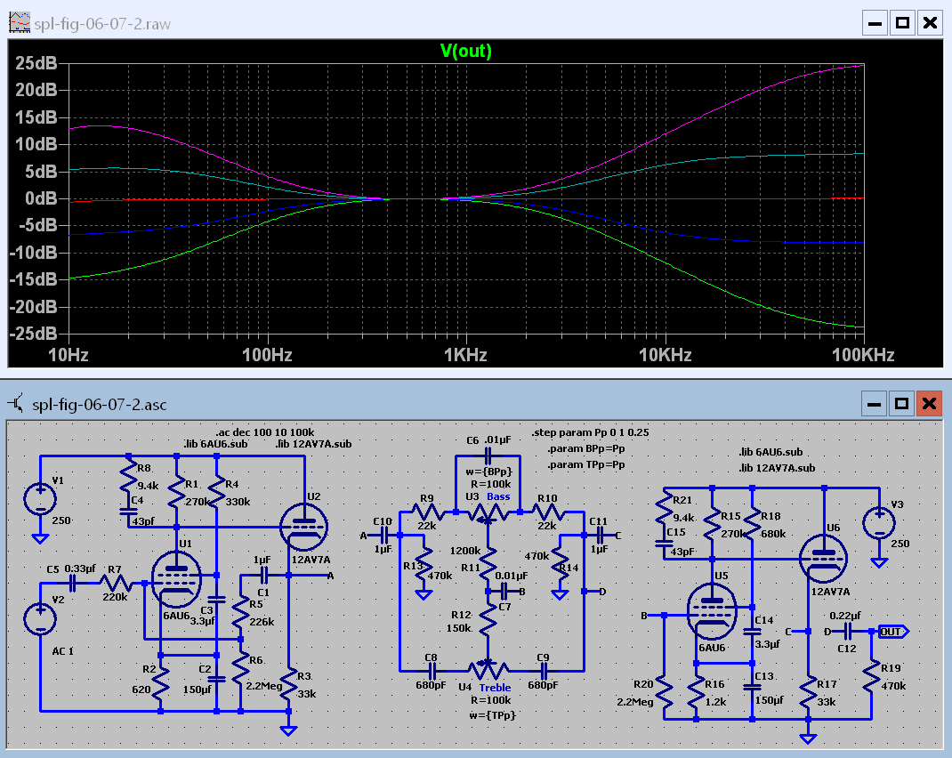
Figure 6.7.2 Changing a resistor on the bass side changed the amount of treble boost and cut.

Hmmm. That didn't do what we expected, did it. Increasing R11 by a factor of 4 should have decreased the bass boost and cut by 12 dB. Instead it increased the amount of treble boost and cut by about 10 dB.

At first glance the graph looks right. But this turns out to be one of those teaching moments. Remember the exercise in the previous lesson where you were fooled by a graph without a scale? It's always important to look at the scale on a graph, not just the curves. Compare figure 6.7.2 with 6.6.1, repeated below to make it easy.

Figure 6.6.1 Repeated for ease of comparison.

The amount of bass boost and cut has changed very little. What did change was the amount of treble boost which caused the graphing routine to adjust the scales on the graph making it look as if the bass boost and cut had been reduced.

So we put R11 back to 300 k ohms and see what other trouble we can get into.

Let's try changing the values of R9 and R10 to reduce the bass boost and cut.
The two resistors in question are now 22 k ohms each. Let's change them to 88 k ohms.

Figure 6.7.3 Changing the resistors on each side of the bass pot.

Well that was interesting. The treble returned to where it had been and the bass boost and cut was reduced but the bass break point was reduced in frequency. If changing the two resistors had done what we really wanted the value of C6 could be decreased to make up for the increase in resistance. Increasing the resistance has the same effect as increasing the capacitance.

Here's a little homework assignment for you. Find the value of C6 that will return the bass breakpoint to where it was.

Measuring the Input Impedance of a Tone Circuit.

Now let's go back to the original values. They can be found in figure 6.6.1.

Close the graph window and make the schematic window full screen. On the left of the passive circuit you will see C10, 1uF. Delete everything to the left of it except V2. Deleting all of that took away the ground for V2 so add one to the lower end of V2.
Add a resistor and connect one end of it to V2. Draw a line (wire) from the other end of this resistor to point A at one end of C10.

Run the simulation. The graph window will be blank.
Left click on the wire between C10 and the resistor you added, Shows as R1 on my system.
You will now see the voltage at this point.
Right click on the right hand vertical axis and click "Don't plot phase".
At the top of the graph window you will see "V(a)" in green. Click on the white banner above the graph window. It will turn blue.
Alt right click on the green text.
A box will open with the characters "V(a)" in it. Make sure the cursor is at the end of the text and type"/I(R1)"
Be sure there aren't any spaces in the string "V(a)/I(R1)". If all is well click OK.
This is simple Ohm's law. Impedance Z = V / I.

Figure 6.8.1 Input impedance of the tone circuit.

You now have the input impedance of the circuit plotted in dB. Right click on the scale on the left and select the "Linear" radio button.
Click OK. You now have the input impedance plotted in ohms versus frequency. You can learn quite a lot by changing the vertical scale to go from 0 to 20 k ohms. Start by right clicking on the scale. You also may want to click the radio button next to Logarithmic.

Save the simulation as spl-fig-06-08-1

Measuring the output impedance of an amplifier.

Now we will examine the output impedance of the three high gain feedback amplifiers and the two unity gain impedance buffers. We can measure the output impedance by connecting a generator to the output of an amplifier and measuring how much current flows. This is usually not recommended when working with real electronics.

If you are continuing work from the previous section press ctl-F4 to close the project. If you have not saved you will be prompted.

You can choose from five different amplifiers to measure their output impedance. Let's start with the worst and the best.
Open the file "Mod_triode_op-amp.asc".
Select "Save as" from the menu and save under the name "spl-fig-06-09-1".

1. If there is a 1 volt AC generator on the left press F7 and move it to the right side of the diagram as shown in figure 6.9.2. Skip step 2.
2. Now add a voltage generator on the right as shown in figure 6.9.1.
   
3. Set its voltage to 1 volt AC.
   
4. Draw a wire to connect its negative end to ground.
   
5. Add a resistor and capacitor as shown in the figure.
   
6. Set the resistor's resistance to 1 ohm and the capacitance of the capacitor to 1000uF.
   
7. If it is not already there, place the following spice directive on the screen. ".ac dec 100 10Hz 100kHz".
   
8. Run it. Connect the scope probe to point "C" or point "A" depending on which circuit you are testing.
   
9. In the graph window alt-right click on V(C) or V(A) in green at the top of the window.
10. A box will open and the character string "V(C)" or "V(A)" will appear.
    
11. The typing cursor should be at the end. If it isn't, move it there.
    
12. In the next step replace the "x" with the number of the newly added resistor.
13. Add the following characters to the end of the string. "/I(Rx)
    
14. Click OK.
15. On the left, draw a line (wire) to connect the grid to ground.
    
16. Note: This is something you really can't do with a real circuit because of nonlinearity in the vacuum tube.
    
17. Save by pressing ctl- S
    
18. Run it.
    
19. Change the left hand scale to linear.
    
20. Click on the label "V(out)/I(c2)" to activate the cursor.
    
21. This will allow you to read the impedance at any frequency.
    
22. Select the graph window and save the graph settings.
    

Open the file "Mod_true-unity-gain,asc".
Select "Save as" from the menu and save under the name "spl-fig-06-09-2". Now go back to step 1 above and complete all steps for this circuit.

Figure 6.9.1 Output impedance of the single triode circuit. The worst.

Figure 6.9.2 Output impedance of the Pentode-Triode circuit. The best.

Figure 6.9.3 Output impedance of the triode-triode circuit. The most practical.

Figure 6.9.4 Output impedance of Cathode follower buffer circuit. Excellent for the purpose.

Figure 6.9.5 Output impedance of Unity Gain Buffer circuit. Impractically Complex.

If you want to go back to the graph settings you saved, they are not loaded automatically.
Right click on the graph.
Select File and Reload Plot Settings from the submenu.

Play Time.

Now that you know how to do it you can patch together any combination of amplifiers and response control circuits to see how well or poorly they work. You also know how to measure the input impedance of the circuit so you can examine the load each circuit places on the driving stage. You now have all the tools you need to have fun with tone controls from early morning to late at night. So get out your toy tractor with the front loader attachment and dig that sand. Have fun. If you come up with something really good, DON'T FORGET TO SAVE THE DRAWING.

If you can honestly checkoff each item on the list under the heading "What you will learn in lesson 6", you can go on to lesson 7, assuming I have written it by then.

This page last updated Friday, May 06, 2022.

Home.