
DIGITAL STORAGE OSCILLOSCOPE
(Tektronix TDS - 210)
By:
Ajay Malhotra and Jason Ogilvie
CNT -1C
CMPH 227
What is an Oscilloscope?
An oscilloscope is an instrument used to measure almost any electrical signal on a two-dimensional graphing display (there are also three-dimensional graphing displays available). In general, oscilloscopes are used to study the characteristics of voltage versus time; displayed on the vertical and horizontal axis respectively. This general-purpose display presents far more information than is available from other test equipment such as frequency counters or multimeters.
Oscilloscopes can help detect the DC and AC components of a signal, the noise level accompanying the signal, and whether the noise is varying with time. It also gives a visual representation of the frequency -- number of cycles per second -- being fed into the oscilloscope. The best feature of the oscilloscope is that all of the above functions are displayed at the same time, thus, eliminating the necessity of doing separate time consuming tests.
What Can You Do With an Oscilloscope?
Oscilloscopes are used by everyone from television repair technicians to physicists. They are indispensable for anyone designing or repairing electronic equipment.
The usefulness of an oscilloscope is not limited to the world of electronics. With the proper transducer, an oscilloscope can measure all kinds of phenomena. A transducer is a device that creates an electrical signal in response to physical stimuli, such as sound, mechanical stress, pressure, light, or heat. For example, a microphone is a transducer.
An automotive engineer uses an oscilloscope to measure engine vibrations. A medical researcher uses an oscilloscope to measure brain waves. The possibilities are endless.
Analog and Digital
Oscilloscopes
Generally, oscilloscopes can
be divided into two categories -- analog and digital. Analog
scopes are the more conventional and bulkier units that use
cathode ray tubes to display waveforms.
An analog oscilloscope
works by applying the measured signal voltage directly to an
electron beam moving across the oscilloscope screen (usually a
cathode-ray tube, CRT). The back side of the screen is treated
with a coating that phosphoresces wherever the electron beam hits
it. The signal voltage deflects the beam up and down
proportionally, tracing the waveform on the screen. The more
frequently the beam hits a particular screen location, the more
brightly it glows. This gives an immediate picture of the
waveform. The CRT limits the range of frequencies an analog scope
can display. At very low frequencies, the signal appears as a
bright, slow-moving dot that's difficult to distinguish as a
waveform. At high frequencies, the CRT's "writing
speed" defines the limit. When the signal frequency exceeds
CRT's writing speed, the display becomes too dim to see. The
fastest analog scopes can display frequencies up to about 1 GHz.
Digital scopes are more compact and lightweight using liquid crystal displays. In contrast to Analog scopes, a digitizing oscilloscope uses an analog-to-digital converter (ADC) to convert the voltage being measured into digital information. The digitizing scope acquires the waveform as a series of samples. It stores these samples until it accumulates enough samples to describe a waveform, and then re-assembles the waveform for viewing on the screen. The conventional digitizing scope is known as a DSO -- digitizing storage oscilloscope. Its display doesn't rely on luminous phosphor; instead, it uses a raster-type screen.
All digitizing scopes
incorporate a microprocessor of some sort. The power of a
processor in a digitizing scope profoundly affects its
capabilities. Since the data is in digital form, it is easy to
have the processor perform some specific tasks on the data. For
instance, we can automatically measure such parameters as time
intervals, rise and fall times, frequency and more. The processor
can also allow such functions as waveform math. Digitizing
storage oscilloscopes allow you to capture and view events that
may happen only once -- "transient" events. Because the
waveform information is in digital form (a series of stored
binary values), it can be analyzed, archived, printed, and
otherwise processed, within the scope itself or by an external
computer. The waveform doesn't need to be continuous; even when
the signal disappears, it can be displayed. However, DSOs have no
real-time intensity grading, therefore they cannot express
varying levels of intensity in the live signal.
How
Digital Storage Oscilloscopes work?

This signal chain shows a typical implementation of a digital storage oscilloscope.
The input signals from the oscilloscope probes are usually attenuated and then buffered before being fed into an ADC(Analog to Digital converter). The attenuation is provided by a passive resistor network. The buffer amplifiers perform level shifting to match the input of the ADC. These buffer amplifiers are required to have between 10 MHz and 500 MHz bandwidth, depending on the speed range of the oscilloscope. The ADCs usually have between 8- and 12-bit resolution with a throughput of about 10 MSPS (Million samples per second) at the low end and a maximum of about 500 MSPS for the fastest oscilloscopes.
Once the signals have been digitized, the digital data is then fed into a FIFO (First-In First-Out) memory. The timing control between the ADC and the FIFO memory is usually performed by a DSP (Digital Signal Processor) and/or a µProcessor. The digital data is fed from the FIFO memory into a high speed video DAC (Digital to Analog converter) which converts the digital data stored in memory back into analog format. The video DAC usually has 8-bit resolution, with an update rate of between 20 MHz and 50 MHz.
Once the data has been
converted back into analog format, it is then fed into the high
voltage X and Y video driver amplifiers that directly drive the
CRT display. Not shown on the block diagram are trigger
comparators (implemented using 10-bit CMOS DACs with 10 µs
settling times) that are used to control trigger level positions.
Sampling Methods
Digitizing oscilloscopes can use either real-time, interpolated real-time, or equivalent-time sampling to collect sample points. Real-time sampling is ideal for signals whose frequency is less than half the scope's maximum sample rate. Here, the oscilloscope can acquire more than enough points in one "sweep" of the waveform to construct an accurate picture (See Figure d below). Note that real time sampling is the only way to capture single-shot transient signals with a digitizing scope.

Figure d: Real-time
Sampling
When measuring high-frequency signals the oscilloscope may not be able to collect enough samples in one sweep. There are two solutions for accurately acquiring signals whose frequency exceeds half the scope's sample rate:
Collect a few sample points of the signal in a single pass (in real-time mode) and use interpolation to fill in the gaps. Interpolation is a processing technique to estimate what the waveform looks like based on a few points
Build a picture of the waveform by acquiring samples from successive cycles of the waveform , assuming the signal repeats itself (equivalent-time sampling mode).
Real-Time Sampling with Interpolation
Digitizing oscilloscopes take discrete samples of the signal which can be displayed. However, it can be difficult to visualize the signal represented as dots, especially because there can be only a few dots representing high frequency portions of the signal. To aid in the visualization of signals, digitizing oscilloscopes typically have interpolation display modes.
In simple terms, interpolation "connects the dots." Using this process, a signal that is sampled only a few times in each cycle can be accurately displayed. However, for accurate representation of the signal, the sample rate should be at least four times the bandwidth of the signal.
Linear interpolation connects sample points with straight lines. This approach is limited to reconstructing straight-edged signals like square waves.
The more versatile sin x/x interpolation connects sample points with curves (See Figure e below). Sin x/x interpolation is a mathematical process in which points are calculated to fill in the time between the real samples.
This form of interpolation lends itself to curved and irregular signal shapes, which are far more common in the real world than pure square waves and pulses. Consequently, sin x /x interpolation is the preferred method for most applications.

Figure e: Linear and Sine Interpolation
Some digitizing oscilloscopes can use equivalent-time sampling to capture very fast repeating signals. Equivalent-time sampling constructs a picture of a repetitive signal by capturing a little bit of information from each repetition. (See Figure f below.) The waveform slowly builds up like a string of lights going on one-by-one. With sequential sampling the points appear from left to right in sequence; with random sampling the points appear randomly along the waveform.

Figure f: Equivalent-time Sampling
Getting started
Before you start working with your oscilloscope, there are a few things you need to do to ensure that your tests will be successful.
Functional check:
The following steps will help you perform a quick functional check to verify your instrument's operating condition:
Now that your oscilloscope has been setup, let us move on to the operating basics of the TDS 210 oscilloscope.
Operating
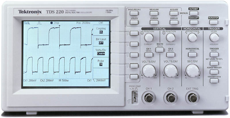
the TDS 210

The front panel of the TDS 210/220 has an easy to use layout. All the controls are similar to the Analog oscilloscopes with the exception of push buttons used in place of throw switches.
Display (Monitor)

The display of the TDS 210 not only shows the waveforms but also provides details about the waveform and control settings.
Horizontal Controls

CH1 and CURSOR 1 POSITION - Controls the channel 1 display and positions cursor 1.
CH2 and CURSOR 2 POSITION - Controls the channel 2 display and positions cursor 2.
MATH MENU - Brings up menu to do math operations on waveforms.
CH1 and CH2 MENU - Displays the channel input menu and toggles the channel display on and off.
VOLTS/DIV (CH1and CH2) - Calibrated scale selection.
Digital Storage Oscilloscope Experiment
Objective: To learn the functions of a digital storage scope that make it a much more useful tool than an analog scope.
Equipment:
1) Tektronix
TDS 210 and manual.
2) Two scope
probes (P6112)
3)
Microprocessor trainer and manual.
Setup Instructions:
(This setup parallels the setup for exercise 10-1 in the microprocessor manual)
1) Plug in and turn on the microprocessor trainer and scope. Connect the two probes to "channel 1" and "channel 2."
2) Connect "channel 1" probe to the data bus line "D0." (The probe goes into the plated hole labeled "D0").
3) Connect "channel 2" probe to IC #12, pin #3. Be careful!
4) Make sure the trigger is set to "channel 1" and the scopes are on DC.
5) Both channels should be set to 2V/division and 1us/division.
6) Set "channel 1" ground at the "0.00 volts" line and position the "channel 2" ground at approximately the "-6.00 volts" line. This should separate the two waveforms enough.
Procedure:
In order to get some
waveforms that can be captured and measured, enter the following
program into the micro trainer:
Press "Fetch
Address"
0800 C3 (Store /
INCR)
0801 00 (Store /
INCR)
0802 08 (Store /
INCR)
Press DECR two times
to get back to 0800 C3 and then press run. This will
provide a "short loop" that can be easily tested with
the D.S.O.. At first glance the waveforms will be moving
quite quickly across the screen. Press the
"Run/Stop" button on the scope. At this point you
should have a display on the screen that looks something like
"figure 1." Notice that the output on
"channel 2" is triggered on the negative going pulse of
"channel 1."
Measuring with Cursors:
Select the cursors with the
Cursor button on the D.S.O.. On the side menu you can
select the voltage or time cursors. Using the same position
knobs as for "channels 1 and 2," select the voltage
cursors and move the two horizontal cursor lines to the points
you want measured.
1) Measure the peak to peak voltage on "channel 1." (Answer: approx. 5.12 V).
2) Using the time cursors (two vertical lines), measure the time for one cycle, and the frequency. (Answer: approx. 5 us and 200 kHz).
3) Referring to
"Figure 1," measure the time frame of "section
A" and then "section B." Notice that
two "section A's" and one "section B" equal
one cycle.
(Answer: approx. 1.5 us for
section A, and 2.0 us for section B).
Digital Storage Oscilloscope Quiz:
Select the best answer(s) for each question.
1) Which feature allows
the user to detect unusual voltage spikes?
A - Sample
B - Peak detect
C - Hardcopy
D - Autoset
2) When the user
wishes to measure a pulse width the best method would be:
A - Select acquire, peak
detect, and read measurement.
B - Select measure, type,
period, and read measurement.
C - Select cursor, time,
place cursors, and read measurement.
D - Select cursor, voltage,
place cursors, and read measurement.
3) Press the ___________ button to get a printout of the displayed waveform.
4) When Averaging out a signal, the four values 4, 16, 64, and 128, represent the number of ___________ taken to make the waveform more _______________.
5) The
_Autoset" function is used to:
A - Sets parameters that were
last saved in memory.
B - Automatically measures
your period and frequency.
C - Stores the most recent
waveform every 5 minutes automatically.
D - Automatically sets the
instrument controls for the best signal.
6) The analog scope uses a liquid crystal display, whereas the digital scope uses the cathode ray tube. True or False?
7) What technology
allows the digital scope to perform tasks such as printing,
saving, and math?
A - The cathode ray tube.
B - The liquid crystal
display.
C - The microprocessor.
D - The Compact Disc.
8) When using the cursor function of the D.S.O., the voltage cursors appear in a ______________ direction, and the time cursors appear in a _____________ direction.
9) Which
button would be selected to change the contrast?
A - Display
B - Math
C - Cursor
D - Utility
10) The "math" function can perform such functions as ___________ waveforms, ____________ waveforms, and/or _____________ waveforms.
(Total of 14 marks).
Answers:
1) B
2) C
3) hardcopy.
4) samples, accurate.
5) D
6) false.
7) C
8) horizontal,
vertical.
9) A
10) subtracting, adding,
inverting.
Interesting Links:
www.tektronix.com (www.tek.com)
www.tmo.hp.com/tmo
